Last active
August 8, 2025 15:40
-
-
Save RodriguezGoldstein/4f09a741c6c09db8d7efb6cc9014d700 to your computer and use it in GitHub Desktop.
option-pricing.ipynb
This file contains hidden or bidirectional Unicode text that may be interpreted or compiled differently than what appears below. To review, open the file in an editor that reveals hidden Unicode characters.
Learn more about bidirectional Unicode characters
| { | |
| "nbformat": 4, | |
| "nbformat_minor": 0, | |
| "metadata": { | |
| "hide_input": false, | |
| "kernelspec": { | |
| "display_name": "Python 3", | |
| "language": "python", | |
| "name": "python3" | |
| }, | |
| "language_info": { | |
| "codemirror_mode": { | |
| "name": "ipython", | |
| "version": 3 | |
| }, | |
| "file_extension": ".py", | |
| "mimetype": "text/x-python", | |
| "name": "python", | |
| "nbconvert_exporter": "python", | |
| "pygments_lexer": "ipython3", | |
| "version": "3.7.4" | |
| }, | |
| "toc": { | |
| "nav_menu": {}, | |
| "number_sections": true, | |
| "sideBar": true, | |
| "skip_h1_title": false, | |
| "toc_cell": false, | |
| "toc_position": {}, | |
| "toc_section_display": "block", | |
| "toc_window_display": false | |
| }, | |
| "colab": { | |
| "name": "option-pricing.ipynb", | |
| "provenance": [], | |
| "collapsed_sections": [], | |
| "include_colab_link": true | |
| } | |
| }, | |
| "cells": [ | |
| { | |
| "cell_type": "markdown", | |
| "metadata": { | |
| "id": "view-in-github", | |
| "colab_type": "text" | |
| }, | |
| "source": [ | |
| "<a href=\"https://colab.research.google.com/gist/RodriguezGoldstein/4f09a741c6c09db8d7efb6cc9014d700/option-pricing.ipynb\" target=\"_parent\"><img src=\"https://colab.research.google.com/assets/colab-badge.svg\" alt=\"Open In Colab\"/></a>" | |
| ] | |
| }, | |
| { | |
| "cell_type": "markdown", | |
| "metadata": { | |
| "id": "iQHMgwZ0xMMw", | |
| "colab_type": "text" | |
| }, | |
| "source": [ | |
| "# Option Pricing via Montecarlo Simulation\n", | |
| "Jose Luis Rodriguez Goldstein\n", | |
| "\n", | |
| "* linkedin.com/in/RodriguezGoldstein\n", | |
| "* github.com/RodriguezGoldstein\n", | |
| "\n", | |
| "## Pricing Call Options \n", | |
| "\n", | |
| "### Monte Carlo Method\n", | |
| "\n", | |
| "https://en.wikipedia.org/wiki/Monte_Carlo_method\n", | |
| "\n", | |
| "Monte Carlo methods (or Monte Carlo experiments) are a broad class of computational algorithms that rely on repeated random sampling to obtain numerical results. \n", | |
| "\n", | |
| "Their essential idea is using randomness to solve problems that might be deterministic in principle. They are often used in physical and mathematical problems and are most useful when it is difficult or impossible to use other approaches. \n", | |
| "\n", | |
| "Monte Carlo methods are mainly used in three distinct problem classes: optimization, numerical integration, and generating draws from a probability distribution.\n", | |
| "\n", | |
| "### Geometric Brownian motion\n", | |
| "\n", | |
| "https://en.wikipedia.org/wiki/Geometric_Brownian_motion\n", | |
| "\n", | |
| "\n", | |
| "\n", | |
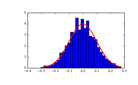
| "### Normal Distribution\n", | |
| "\n", | |
| "https://docs.scipy.org/doc/numpy-1.12.0/reference/generated/numpy.random.normal.html#numpy.random.normal\n", | |
| "\n", | |
| "\n", | |
| "\n", | |
| "### Tesla Option Prices\n", | |
| "\n", | |
| "https://finance.yahoo.com/quote/TSLA/options\n", | |
| "\n", | |
| "\n" | |
| ] | |
| }, | |
| { | |
| "cell_type": "markdown", | |
| "metadata": { | |
| "id": "26YU40G8xMMy", | |
| "colab_type": "text" | |
| }, | |
| "source": [ | |
| "## Background\n", | |
| "\n", | |
| "Monte Carlo methods vary, but tend to follow a particular pattern:\n", | |
| "\n", | |
| "1. Define a domain of possible inputs\n", | |
| "2. Generate inputs randomly from a probability distribution over the domain\n", | |
| "3. Perform a deterministic computation on the inputs\n", | |
| "4. Aggregate the results\n", | |
| "\n", | |
| "Assume that asset prices follow a geometric Brownian motion. Since this is a random process in which a logarithm of the random variable follows a normal distribution then the assets prices are distributed over a lognormal distribution making possible to use Monte Carlo method to generate random inputs.\n", | |
| "\n", | |
| "Give an asset ($S$) at time ($t$) we can estimate the asset price at time ($T$) as follows:\n", | |
| "\n", | |
| "$$S_T = S_t e^{(r-\\frac{1}{2}\\sigma^2)(T-t)+\\sigma\\sqrt{T-t} \\epsilon}$$\n", | |
| "\n", | |
| "$r$: Risk free interest rate \n", | |
| "\n", | |
| "$\\sigma$ (volatility): Annualized standard deviation of a stock's returns.\n", | |
| "\n", | |
| "$(T-t)$: Annualized time to maturity\n", | |
| "\n", | |
| "$S_t$: Underlying asset price\n", | |
| "\n", | |
| "$\\epsilon$: Random value that follows a normal distribution with mean of 0.0 and standard deviation of 1.0\n", | |
| "\n", | |
| "Now we can use Monte Carlo method as follows:\n", | |
| "\n", | |
| "1. Draw a random value from the normal distribution\n", | |
| "2. Estimate the asset price for that draw\n", | |
| "3. If the payoff ($S - K)$ is great than zero keep store the result\n", | |
| "4. To calculate the final price We need to discount the sum of the estimates divide by the number of simulations\n" | |
| ] | |
| }, | |
| { | |
| "cell_type": "code", | |
| "metadata": { | |
| "id": "zhrDP6HdxMMz", | |
| "colab_type": "code", | |
| "colab": {} | |
| }, | |
| "source": [ | |
| "import datetime\n", | |
| "import numpy as np\n", | |
| "import pandas as pd\n", | |
| "import multiprocessing as mp" | |
| ], | |
| "execution_count": 0, | |
| "outputs": [] | |
| }, | |
| { | |
| "cell_type": "code", | |
| "metadata": { | |
| "id": "1qGLBdFlxMM3", | |
| "colab_type": "code", | |
| "colab": {} | |
| }, | |
| "source": [ | |
| "S = 901.00 # underlying price\n", | |
| "sigma = 0.8424 # vol of 84.24%\n", | |
| "r = 0.0142 # rate of 0.142% (12 Month GB12:GOV)\n", | |
| "expiration = datetime.date(2020,3,20)\n", | |
| "today = datetime.date(2020,2,24)\n", | |
| "T = (expiration - today).days / 365.0\n", | |
| "K = 950.00\n", | |
| "N = 900000" | |
| ], | |
| "execution_count": 0, | |
| "outputs": [] | |
| }, | |
| { | |
| "cell_type": "markdown", | |
| "metadata": { | |
| "id": "QoEUJYf8xMM6", | |
| "colab_type": "text" | |
| }, | |
| "source": [ | |
| "## Call Option Asset Simulation" | |
| ] | |
| }, | |
| { | |
| "cell_type": "code", | |
| "metadata": { | |
| "id": "JDQllFHSxMM7", | |
| "colab_type": "code", | |
| "colab": {} | |
| }, | |
| "source": [ | |
| "def __assetPrice__(S, sigma, r, T, epsilon):\n", | |
| " price = S * np.exp((r - 0.5 * sigma**2) * T + (sigma * np.sqrt(T) * epsilon))\n", | |
| " return price\n", | |
| "\n", | |
| "def call_option_table(S, K, sigma, r, T, N):\n", | |
| " rf_rate = np.exp(-r * T)\n", | |
| " mc = [] \n", | |
| " for i in range(N):\n", | |
| " epsilon = np.random.normal(0, 1)\n", | |
| " d = {}\n", | |
| " d['epsilon'] = epsilon\n", | |
| " price = __assetPrice__(S, sigma, r, T, epsilon)\n", | |
| " d['strike_price'] = K\n", | |
| " d['asset_price'] = price\n", | |
| " call_payoff = price - K\n", | |
| " if call_payoff > 0:\n", | |
| " d['payoff'] = call_payoff\n", | |
| " d['discounted'] = rf_rate * call_payoff / N\n", | |
| " else:\n", | |
| " d['payoff'] = 0\n", | |
| " d['discounted'] = 0\n", | |
| " mc.append(d)\n", | |
| " df = pd.DataFrame.from_dict(mc)\n", | |
| " return df" | |
| ], | |
| "execution_count": 0, | |
| "outputs": [] | |
| }, | |
| { | |
| "cell_type": "code", | |
| "metadata": { | |
| "id": "KEk9A6tHxMM-", | |
| "colab_type": "code", | |
| "outputId": "2e27c852-404e-48af-9242-dc14f93da71a", | |
| "colab": {} | |
| }, | |
| "source": [ | |
| "table = call_option_table(S, K, sigma, r, T, N)\n", | |
| "table.head(6)" | |
| ], | |
| "execution_count": 0, | |
| "outputs": [ | |
| { | |
| "output_type": "execute_result", | |
| "data": { | |
| "text/html": [ | |
| "<div>\n", | |
| "<style scoped>\n", | |
| " .dataframe tbody tr th:only-of-type {\n", | |
| " vertical-align: middle;\n", | |
| " }\n", | |
| "\n", | |
| " .dataframe tbody tr th {\n", | |
| " vertical-align: top;\n", | |
| " }\n", | |
| "\n", | |
| " .dataframe thead th {\n", | |
| " text-align: right;\n", | |
| " }\n", | |
| "</style>\n", | |
| "<table border=\"1\" class=\"dataframe\">\n", | |
| " <thead>\n", | |
| " <tr style=\"text-align: right;\">\n", | |
| " <th></th>\n", | |
| " <th>epsilon</th>\n", | |
| " <th>strike_price</th>\n", | |
| " <th>asset_price</th>\n", | |
| " <th>payoff</th>\n", | |
| " <th>discounted</th>\n", | |
| " </tr>\n", | |
| " </thead>\n", | |
| " <tbody>\n", | |
| " <tr>\n", | |
| " <td>0</td>\n", | |
| " <td>1.361872</td>\n", | |
| " <td>950.0</td>\n", | |
| " <td>1188.469729</td>\n", | |
| " <td>238.469729</td>\n", | |
| " <td>0.000265</td>\n", | |
| " </tr>\n", | |
| " <tr>\n", | |
| " <td>1</td>\n", | |
| " <td>-0.899141</td>\n", | |
| " <td>950.0</td>\n", | |
| " <td>721.942237</td>\n", | |
| " <td>0.000000</td>\n", | |
| " <td>0.000000</td>\n", | |
| " </tr>\n", | |
| " <tr>\n", | |
| " <td>2</td>\n", | |
| " <td>1.101115</td>\n", | |
| " <td>950.0</td>\n", | |
| " <td>1122.073827</td>\n", | |
| " <td>172.073827</td>\n", | |
| " <td>0.000191</td>\n", | |
| " </tr>\n", | |
| " <tr>\n", | |
| " <td>3</td>\n", | |
| " <td>-0.799129</td>\n", | |
| " <td>950.0</td>\n", | |
| " <td>738.037223</td>\n", | |
| " <td>0.000000</td>\n", | |
| " <td>0.000000</td>\n", | |
| " </tr>\n", | |
| " <tr>\n", | |
| " <td>4</td>\n", | |
| " <td>-1.525348</td>\n", | |
| " <td>950.0</td>\n", | |
| " <td>628.846705</td>\n", | |
| " <td>0.000000</td>\n", | |
| " <td>0.000000</td>\n", | |
| " </tr>\n", | |
| " <tr>\n", | |
| " <td>5</td>\n", | |
| " <td>0.694368</td>\n", | |
| " <td>950.0</td>\n", | |
| " <td>1025.832651</td>\n", | |
| " <td>75.832651</td>\n", | |
| " <td>0.000084</td>\n", | |
| " </tr>\n", | |
| " </tbody>\n", | |
| "</table>\n", | |
| "</div>" | |
| ], | |
| "text/plain": [ | |
| " epsilon strike_price asset_price payoff discounted\n", | |
| "0 1.361872 950.0 1188.469729 238.469729 0.000265\n", | |
| "1 -0.899141 950.0 721.942237 0.000000 0.000000\n", | |
| "2 1.101115 950.0 1122.073827 172.073827 0.000191\n", | |
| "3 -0.799129 950.0 738.037223 0.000000 0.000000\n", | |
| "4 -1.525348 950.0 628.846705 0.000000 0.000000\n", | |
| "5 0.694368 950.0 1025.832651 75.832651 0.000084" | |
| ] | |
| }, | |
| "metadata": { | |
| "tags": [] | |
| }, | |
| "execution_count": 4 | |
| } | |
| ] | |
| }, | |
| { | |
| "cell_type": "markdown", | |
| "metadata": { | |
| "id": "LcRCpPtexMNC", | |
| "colab_type": "text" | |
| }, | |
| "source": [ | |
| "## For Loop Approach" | |
| ] | |
| }, | |
| { | |
| "cell_type": "code", | |
| "metadata": { | |
| "id": "UfwLwnEIxMNC", | |
| "colab_type": "code", | |
| "colab": {} | |
| }, | |
| "source": [ | |
| "def __assetPrice__(S, sigma, r, T):\n", | |
| " epsilon = np.random.normal(0, 1)\n", | |
| " price = S * np.exp((r - 0.5 * sigma**2) * T + (sigma * np.sqrt(T) * epsilon))\n", | |
| " return price\n", | |
| "\n", | |
| "def pricing_option_for(S, K, sigma, r, T, N):\n", | |
| " rf_rate = np.exp(-r * T)\n", | |
| " call_payoff = 0 \n", | |
| " for i in range(N):\n", | |
| " price = __assetPrice__(S, sigma, r, T)\n", | |
| " payoff = price - K\n", | |
| " if payoff > 0:\n", | |
| " call_payoff += payoff\n", | |
| " price = rf_rate * call_payoff / float(N)\n", | |
| " return price" | |
| ], | |
| "execution_count": 0, | |
| "outputs": [] | |
| }, | |
| { | |
| "cell_type": "markdown", | |
| "metadata": { | |
| "id": "aMpbC5edxMNF", | |
| "colab_type": "text" | |
| }, | |
| "source": [ | |
| "## List Comprehensions Approach" | |
| ] | |
| }, | |
| { | |
| "cell_type": "code", | |
| "metadata": { | |
| "id": "suC1OiMExMNG", | |
| "colab_type": "code", | |
| "colab": {} | |
| }, | |
| "source": [ | |
| "def __assetPrice__(S, sigma, r, T):\n", | |
| " epsilon = np.random.normal(0, 1)\n", | |
| " price = S * np.exp((r - 0.5 * sigma**2) * T + (sigma * np.sqrt(T) * epsilon))\n", | |
| " return price\n", | |
| " \n", | |
| "def pricing_option_list(S, K, sigma, r, T, N):\n", | |
| " rf_rate = np.exp(-r * T)\n", | |
| " call_payoff = [ __assetPrice__(S, sigma, r, T) - K for i in range(N) ] \n", | |
| " price = rf_rate * sum(filter(lambda x: x>0, call_payoff)) / float(N)\n", | |
| " return price" | |
| ], | |
| "execution_count": 0, | |
| "outputs": [] | |
| }, | |
| { | |
| "cell_type": "markdown", | |
| "metadata": { | |
| "id": "ZnPpGk7kxMNJ", | |
| "colab_type": "text" | |
| }, | |
| "source": [ | |
| "## Multiprocessing Approach" | |
| ] | |
| }, | |
| { | |
| "cell_type": "code", | |
| "metadata": { | |
| "id": "K9zMYP85xMNK", | |
| "colab_type": "code", | |
| "colab": {} | |
| }, | |
| "source": [ | |
| "class PricingOptionMP:\n", | |
| " \"\"\"\n", | |
| " Asset Price Simulation\n", | |
| " \"\"\"\n", | |
| " def __init__(self, S, K, sigma, r, T):\n", | |
| " self.S = S\n", | |
| " self.K = K\n", | |
| " self.sigma = sigma\n", | |
| " self.r = r\n", | |
| " self.T = T\n", | |
| " self.rf_rate = np.exp(-r * T)\n", | |
| " \n", | |
| " def __price__(self,*args):\n", | |
| " epsilon = np.random.normal(0, 1)\n", | |
| " estimate = S * np.exp((r - 0.5 * sigma**2) * T + (sigma * np.sqrt(T) * epsilon))\n", | |
| " return estimate - self.K\n", | |
| "\n", | |
| " def call_option(self, N):\n", | |
| " with mp.Pool() as pool:\n", | |
| " call_payoff = pool.map(self.__price__, range(N))\n", | |
| " price = self.rf_rate * sum(filter(lambda x: x>0, call_payoff)) / float(N)\n", | |
| " return price" | |
| ], | |
| "execution_count": 0, | |
| "outputs": [] | |
| }, | |
| { | |
| "cell_type": "markdown", | |
| "metadata": { | |
| "id": "iVZPy9xLxMNM", | |
| "colab_type": "text" | |
| }, | |
| "source": [ | |
| "\n", | |
| "\n", | |
| "# Benchmarks\n", | |
| "\n" | |
| ] | |
| }, | |
| { | |
| "cell_type": "code", | |
| "metadata": { | |
| "id": "bC8e1Wt-xMNN", | |
| "colab_type": "code", | |
| "colab": {} | |
| }, | |
| "source": [ | |
| "num_simulations = 5000000" | |
| ], | |
| "execution_count": 0, | |
| "outputs": [] | |
| }, | |
| { | |
| "cell_type": "markdown", | |
| "metadata": { | |
| "id": "0ycCDe-DxMNQ", | |
| "colab_type": "text" | |
| }, | |
| "source": [ | |
| "## For Loop Execution Time" | |
| ] | |
| }, | |
| { | |
| "cell_type": "code", | |
| "metadata": { | |
| "id": "tflqS7x2xMNR", | |
| "colab_type": "code", | |
| "outputId": "6acef72a-6ccd-4dd6-cfa5-8b742d429990", | |
| "colab": {} | |
| }, | |
| "source": [ | |
| "%%time \n", | |
| "pricing_option_for(S, K, sigma, r, T, N=num_simulations)" | |
| ], | |
| "execution_count": 0, | |
| "outputs": [ | |
| { | |
| "output_type": "stream", | |
| "text": [ | |
| "CPU times: user 27.8 s, sys: 44.5 ms, total: 27.8 s\n", | |
| "Wall time: 27.9 s\n" | |
| ], | |
| "name": "stdout" | |
| }, | |
| { | |
| "output_type": "execute_result", | |
| "data": { | |
| "text/plain": [ | |
| "59.47061154205644" | |
| ] | |
| }, | |
| "metadata": { | |
| "tags": [] | |
| }, | |
| "execution_count": 11 | |
| } | |
| ] | |
| }, | |
| { | |
| "cell_type": "markdown", | |
| "metadata": { | |
| "id": "Pmrp4pHXxMNT", | |
| "colab_type": "text" | |
| }, | |
| "source": [ | |
| "## List Comprehensions Execution Time" | |
| ] | |
| }, | |
| { | |
| "cell_type": "code", | |
| "metadata": { | |
| "id": "p105MoRdxMNU", | |
| "colab_type": "code", | |
| "outputId": "a8140b00-da17-490d-9a2a-dafe0d7e0f44", | |
| "colab": {} | |
| }, | |
| "source": [ | |
| "%%time\n", | |
| "pricing_option_list(S, K, sigma, r, T, N=num_simulations)" | |
| ], | |
| "execution_count": 0, | |
| "outputs": [ | |
| { | |
| "output_type": "stream", | |
| "text": [ | |
| "CPU times: user 27.9 s, sys: 135 ms, total: 28 s\n", | |
| "Wall time: 28.1 s\n" | |
| ], | |
| "name": "stdout" | |
| }, | |
| { | |
| "output_type": "execute_result", | |
| "data": { | |
| "text/plain": [ | |
| "59.36738615428871" | |
| ] | |
| }, | |
| "metadata": { | |
| "tags": [] | |
| }, | |
| "execution_count": 14 | |
| } | |
| ] | |
| }, | |
| { | |
| "cell_type": "markdown", | |
| "metadata": { | |
| "id": "WyVWEqYLxMNW", | |
| "colab_type": "text" | |
| }, | |
| "source": [ | |
| "## Multiprocessing Execution Time" | |
| ] | |
| }, | |
| { | |
| "cell_type": "code", | |
| "metadata": { | |
| "id": "6Norlz6sxMNX", | |
| "colab_type": "code", | |
| "outputId": "71ae561b-9fe6-42a0-eb87-56df3cf21e06", | |
| "colab": {} | |
| }, | |
| "source": [ | |
| "%%time\n", | |
| "estimate = PricingOptionMP(S, K, sigma, r, T)\n", | |
| "estimate.call_option(N = num_simulations)" | |
| ], | |
| "execution_count": 0, | |
| "outputs": [ | |
| { | |
| "output_type": "stream", | |
| "text": [ | |
| "CPU times: user 3.92 s, sys: 406 ms, total: 4.33 s\n", | |
| "Wall time: 10.1 s\n" | |
| ], | |
| "name": "stdout" | |
| }, | |
| { | |
| "output_type": "execute_result", | |
| "data": { | |
| "text/plain": [ | |
| "59.41783738885634" | |
| ] | |
| }, | |
| "metadata": { | |
| "tags": [] | |
| }, | |
| "execution_count": 16 | |
| } | |
| ] | |
| }, | |
| { | |
| "cell_type": "code", | |
| "metadata": { | |
| "id": "-Yq4zpamxMNZ", | |
| "colab_type": "code", | |
| "colab": {} | |
| }, | |
| "source": [ | |
| "" | |
| ], | |
| "execution_count": 0, | |
| "outputs": [] | |
| } | |
| ] | |
| } |
Author
Sign up for free
to join this conversation on GitHub.
Already have an account?
Sign in to comment
Example of Tesla Option prices from Schwab