Last active
July 3, 2025 14:39
-
-
Save guohaiping/a28574744a887269a5a2ba4bed56c65d to your computer and use it in GitHub Desktop.
CBuilder_Tutorial
This file contains hidden or bidirectional Unicode text that may be interpreted or compiled differently than what appears below. To review, open the file in an editor that reveals hidden Unicode characters.
Learn more about bidirectional Unicode characters
| # CBuilder FX Tutorial | |
| RSCAD®Fx | |
| # Table of Contents | |
| 1 MULTIPLE INPUT ADDER 1 | |
| 1.1 Introduction 1 1.2 Create a New Component. 1 1.3 Create the Required Parameters 2 1.5 Draw the Graphics. 5 1.6 Add the IO Points. 11 1.7 Adding the Model Code. 14 1.8 Sample $^{\prime}C^{\prime}$ Code for the Multiple Input Adder. 15 2 INTEGRATOR. 1 2.1 Introduction. 1 2.2 draw Graphics and Add Parameters. 2 2.3 Adding the Model Code. 2 2.4 Sample $^{\prime}C^{\prime}$ Code for an Integrator. 3 2.5 Add a Reset Input to the Integrator. 4 3 VARIABLE CAPACITOR. 1 3.1 Introduction. 1 3.2 Capacitor. 2 3.3 Draw Graphics and Add Parameters. 3 3.4 Adding the Model Code. 4 3.5 Adding an Optionally Monitored Variable. 6 4 MULTI- MASS SYSTEM. 1 4.1 Introduction. 1 4.2 Single Mass Rotating About And Axis. 2 4.2.1 Equations Of Motion Representing A Single Mass Rotating About An Axis. 2 4.3 Damping. 4 4.4 Two Rotating Masses Coupled By A Shaft. 6 4.4.1 Equations Of Motion For 2 Rotating Masses Coupled By A Shaft. 6 4.5 Multi- Mass Model Using Matrix Formulation. 9 4.6 Multi- Mass Model Algorithm. 11 4.7 Model Development Using C- Builder. 11 4.7.1 Conceptual Layout Of The New Component. 11 | |
| 4.7.2 Component Icon Creation In C- Builder (Graphics & Nodes) 12 4.7.3 Define User Supplied Data Menus (Parameters) 12 4.7.4 Write Data Preparation Portion Of The 'C' Program 12 4.7.5 Write 'C' Code To Implement The Algorithm 12 4.7.6 Test Newly Developed Model 12 4.7.7 Conceptual Layout Of The New Component 12 4.7.8 Component Icon Creation In C- Builder 15 4.7.9 Add Parameter Entry Menus 20 4.7.10 Write Data Preparation Portion Of The 'C' Program 22 4.7.11 Write 'C' Code To Implement The Algorithm 25 4.7.12 Test Newly Developed Model 30 | |
| 4.8 References 31 | |
| 5 MULTI- THREAD COMPONENT 1 | |
| 5.1 Introduction 1 5.2 Multi- Function Relays 2 5.3 Multi- Thread Component 2 5.4 Model Development using CBuilder 3 5.5 Multi- Thread Model Algorithm 12 5.6 Multi- Thread Static Section 13 5.7 Multi- Thread Ram section 14 5.8 Multi- Thread Code Section 17 | |
| 6 PMU SHELL COMPONENT 1 | |
| 6.1 Introduction 1 6.2 Phasor Measurement Unit 1 6.3 Model Development using CBuilder 2 6.4 PMU Shell Component 3 6.5 Load PMU Shell into CBuilder 3 6.6 PMU Shell Algorithm 4 6.7 C Code Sections 6 6.8 References 11 | |
| 7 GENERATOR CONTROL BLOCK 1 | |
| 7.1 Introduction 1 7.2 Draw Graphics and Add Parameters 1 | |
| 7.3 Adding the Model Code 27.4 Sample 'C' Code for the DC1 Type Exciter 37.5 Data Preparation and Initialization 117.6 Add an internal Slider 137.7 Add Code for realpole Function 157.8 Add Code leadlag Function 157.9 Add Code for washOut Function 157.10 Add Code for Saturation Function 167.11 Adding the Code 167.12 Add a Dial to Select InterNal Variables for Monitoring 207.13 Add a Generic Output 217.14 Add Monitoring Code 218 SIMPLE TRANSFORMER 18.1 Introduction 18.2 Theory 18.2.1 Modelling a Transformer 18.2.2 RTDS Solution Algorithm 48.2.3 Integrating the Transformer Model into the RTDS Solution Algorithm 58.2.4 Generalizing the Transformer Equations 98.3 Draw Graphics and Add Parameters 118.4 Adding the Model Code 128.5 Basic Algorithm 138.6 References 199 MULTIPLIER WITH COMPLEX NUMBERS AS INPUTS 19.1 Introduction 19.2 Create the Required Parameters 19.3 Add the IO Points 29.4 Adding the Model Code 39.5 Sample 'C' Code for the Multiple Input Multiplier with Complex Number Inputs 4 | |
| # 1 MULTIPLE INPUT ADDER | |
| # 1.1 INTRODUCTION | |
| Simple use of the Component Builder (CBuilder) module in RSCAD FX is going to be detailed in this chapter. CBuilder module lets users' create their own components for RSCAD. The CBuilder FX includes a conversion utility to convert CBuilder components created in older versions of RSCAD into RSCAD FX. | |
| In this tutorial chapter, the user will build an adder component that can add or subtract two or three inputs. This adder will be able to accept real type inputs. | |
| # 1.2 CREATE A NEW COMPONENT | |
| Start RSCAD, Open "Component Builder" from the Launch menu. Select "New Component" at the welcome dialog. Select "Control" for the Component Type | |
| 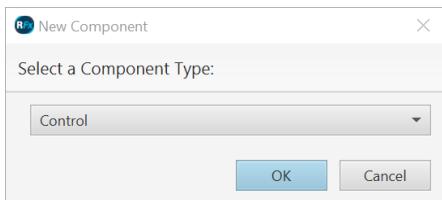 | |
| Figure 1.1: Set Initial Options Menu | |
| The CBuilder module will appear as shown in Figure 1.2. | |
| 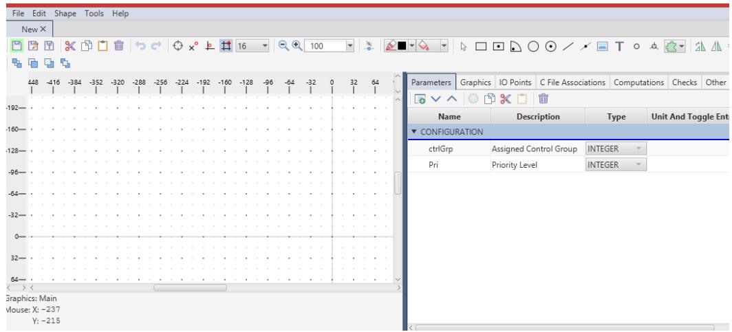 | |
| Figure 1.2: CBuilder FX | |
| - Save the component as "tutorialc". It will have a .def file extension. | |
| # 1.3 CREATE THE REQUIRED PARAMETERS | |
| The required parameters are going to be added into a new section. Each section will appear as a separate tab in Draft when you edit the parameters of the component. The "New Section" and "New parameter" buttons are identified in the toolbar in Figure 1.3. | |
| - Select the Parameters tab. | |
| 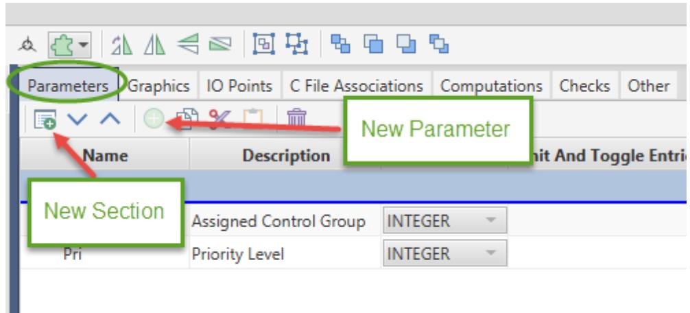 | |
| Figure 1.3: Parameters Tab | |
| - Add a new section titled "addercontrol" | |
| - New parameters will be added at the insertion point, which is a blue line in the table. By clicking on a section header, the insertion point will be placed at the end of that section. Click on a existing parameter and the insertion point will be placed immediately after that parameter. Before adding a new parameter ensure that the | |
| # insertion point is in the section "addercontrol". | |
| 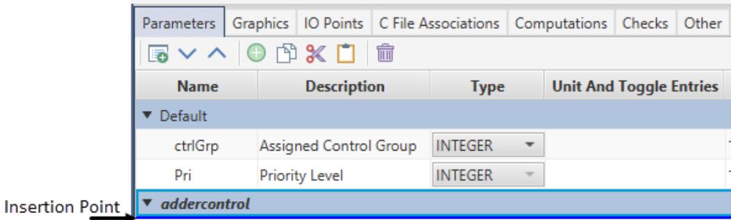 | |
| Figure 1.4:Insertion Point | |
| A number of fields must be entered to define each new parameters. Add the following parameters to the newly created section. | |
| # Parameter #1 | |
| <table><tr><td>Name</td><td>numInputs</td></tr><tr><td>Description</td><td>Number of Inputs</td></tr><tr><td>Type</td><td>INTEGER</td></tr><tr><td>Unit And Toggle Entries</td><td><leave blank></td></tr><tr><td>Value</td><td>2</td></tr><tr><td>Min</td><td>2</td></tr><tr><td>Max</td><td>3</td></tr></table> | |
| </leave> | |
| # Parameter #2 | |
| <table><tr><td>Name</td><td>sign1</td></tr><tr><td>Description</td><td>Sign of Input 1</td></tr><tr><td>Type</td><td>TOGGLE</td></tr><tr><td>Unit And Toggle Entries</td><td>Add;Subtract</td></tr><tr><td>Value</td><td>Add</td></tr><tr><td>Min</td><td>0</td></tr><tr><td>Max</td><td>1</td></tr></table> | |
| The toggle entries must be entered separated by semicolon ";" | |
| The parameter sign1 will be assigned a value of 0 if the "Add" toggle entry is selected, it will be assigned a value of 1 if "Subtract" is selected. | |
| Inputs sign2 and sign3 must also be added as parameters. They can be added manually or the existing sign1 parameter can be copied, pasted and modified. Note the sign3 is conditionally enabled. | |
| # Parameter #3 | |
| Parameter #4 | |
| <table><tr><td>Name</td><td>sign2</td></tr><tr><td>Description</td><td>Sign of Input 2</td></tr><tr><td>Type</td><td>TOGGLE</td></tr><tr><td>Unit And Toggle Entries</td><td>Add;Subtract</td></tr><tr><td>Value</td><td>Add</td></tr><tr><td>Min</td><td>0</td></tr><tr><td>Max</td><td>1</td></tr></table> | |
| <table><tr><td>Name</td><td>sign3</td></tr><tr><td>Description</td><td>Sign of Input 3</td></tr><tr><td>Type</td><td>TOGGLE</td></tr><tr><td>Unit And Toggle Entries</td><td>Add;Subtract</td></tr><tr><td>Value</td><td>Add</td></tr><tr><td>Min</td><td>0</td></tr><tr><td>Max</td><td>1</td></tr><tr><td>Enabled Condition</td><td>numInputs&gt;2</td></tr></table> | |
| # 1.4 DRAW THE GRAPHICS | |
| The main toolbar shown in Figure 1.5 contains tools for drawing the component's graphics. | |
| 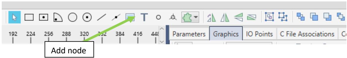 | |
| Figure 1.5: Tools For Drawing Component Graphics | |
| There are four sections of graphics for each component. The user can switch between these graphics section using a dropdown in the Graphics tab which is shown in Figure 1.6. 1. Main | |
| 1. Main | |
| 2. Tiny3. Library4. Loadflow | |
| Note: All four sections should be present for all components. The later chapters will not further discuss the tiny and library graphics, but it is the users' responsibility to make sure those sections are present and to follow the guidelines presented in this chapter. | |
| 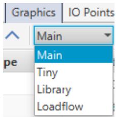 | |
| Figure 1.6: Graphics Dropdown Menu | |
| In the toolbar, the "Add macro" dropdown menu has a collection of basic shapes that can make the drawing process efficient. | |
| 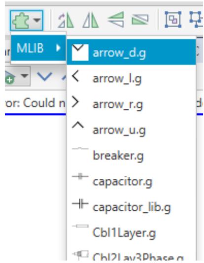 | |
| Figure 1.7: Available Macros | |
| # 1.4.1 Main Graphics | |
| The goal is to draw a component icon that looks similar to Figure 1.8. | |
| 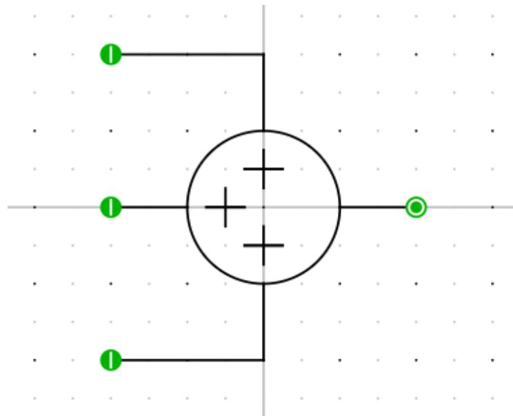 | |
| Figure 1.8: Finished Component Icon | |
| Several snap- to options exist to make drawing component graphics easier. There are a number of helpful toolbar buttons as seen in Figure 1.9. In the figure the option "Snap to Grid" is selected. This will allow the graphical objects to snap to the points on the grid. A dropdown can be used to set the grid point spacing as small as 2 pixels, or as large as 32 pixels. The user can also choose to not snap to grid. | |
| 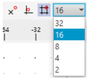 | |
| Figure 1.9: Grid Options | |
| - Start by drawing the unconditional graphics. The graphics can be drawn by using the drawing tools at the top toolbar of the main window. Ensure that the graphics are drawn near the center of the canvas (indicated by the intersecting lines). | |
| 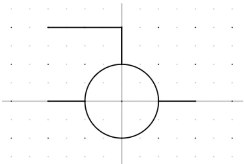 | |
| Figure 1.10: Drawing the Unconditional Graphics | |
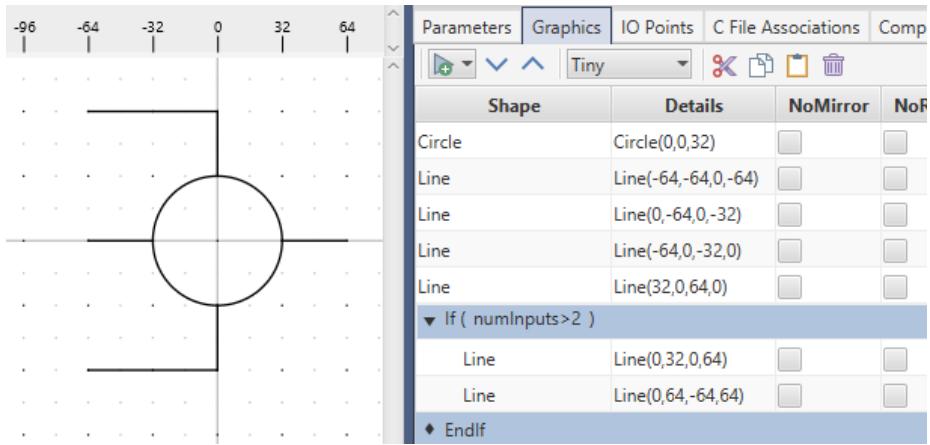
| - Select the "Graphics" tab. With the unconditional graphics drawn, the graphics section should appear similar to Figure 1.11. | |
| 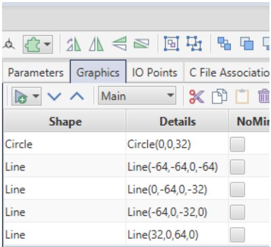 | |
| Figure 1.11: Unconditional Graphics | |
| Please refer to Figure 1.12 and Figure 1.13 for the steps below. | |
| - Add a new "If" graphics condition. This condition will be used to change the look of the icon depending on the number of inputs. | |
| 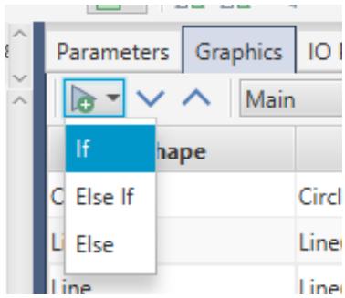 | |
| Figure 1.12: Selecting "If" from Add Condition Drop Down Menu | |
| Enter the condition sign1 $= = 0$ in the box provided. | |
| Enter the condition sign1 $= = 0$ in the box provided.- Ensure the insertion point is located within the new 'sign1 $= = 0$ ' (Add) condition. This can be done by clicking on the condition. Any graphics added will now be placed within the 'If' condition.- Draw a '+' sign with lines at the 12 o'clock position of the inside of the circle using the line tool to indicate the sign of input1. - Ensure the insertion point is inside the 'sign1 $= = 0$ ' condition. Add a new 'Else' condition. The insertion point should now be inside the Else condition (Subtract).- Draw a '+' sign over the '+' sign. The graphics for the minus sign should now appear under the Else condition. Note that the shapes inside each If/Else can be shown or hidden by clicking on the triangle beside the If/Else.- Move the insertion point outside of the conditions. This can be done by clicking on a graphical object in the tree that is not inside a condition. Repeat the above steps to create conditional graphics for 'sign2 $= = 0$ ', except put the graphics at the 9 o'clock position of the circle.- Move the insertion point outside of the conditions and add a new 'If condition'.- Enter condition 'numInputs>2'.- Ensure the insertion point is inside the 'numInputs>2' condition and draw the third input lines.- Ensure the insertion point is still inside 'numInputs>2' and add the condition 'sign3 $= = 0$ '.- Ensure the insertion point is now inside the 'sign3 $= = 0$ ' condition and add the conditional '+' and '- graphics described in previous steps at the 6 o'clock position of the circle. | |
| The icon should now appear similar to Figure 1.13. | |
| 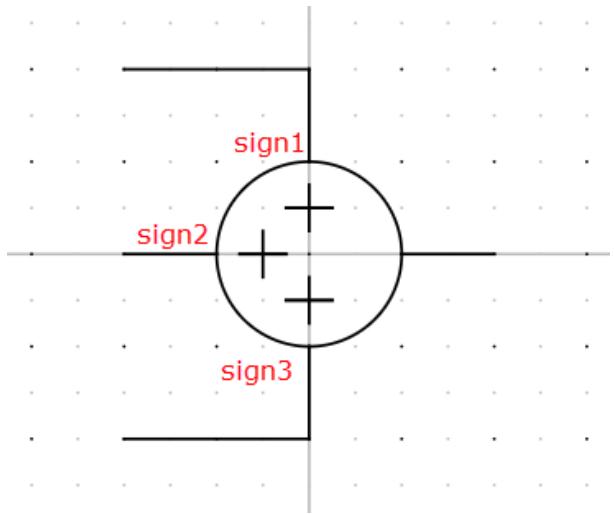 | |
| Figure 1.13: Component Icon | |
| The conditional graphics section in the graphics tab would appear as: | |
| 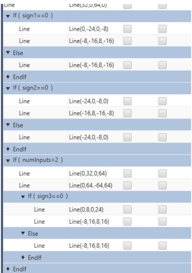 | |
| Figure 1.14: Conditional Section of the Graphics | |
| # 1.4.2 Tiny Graphics | |
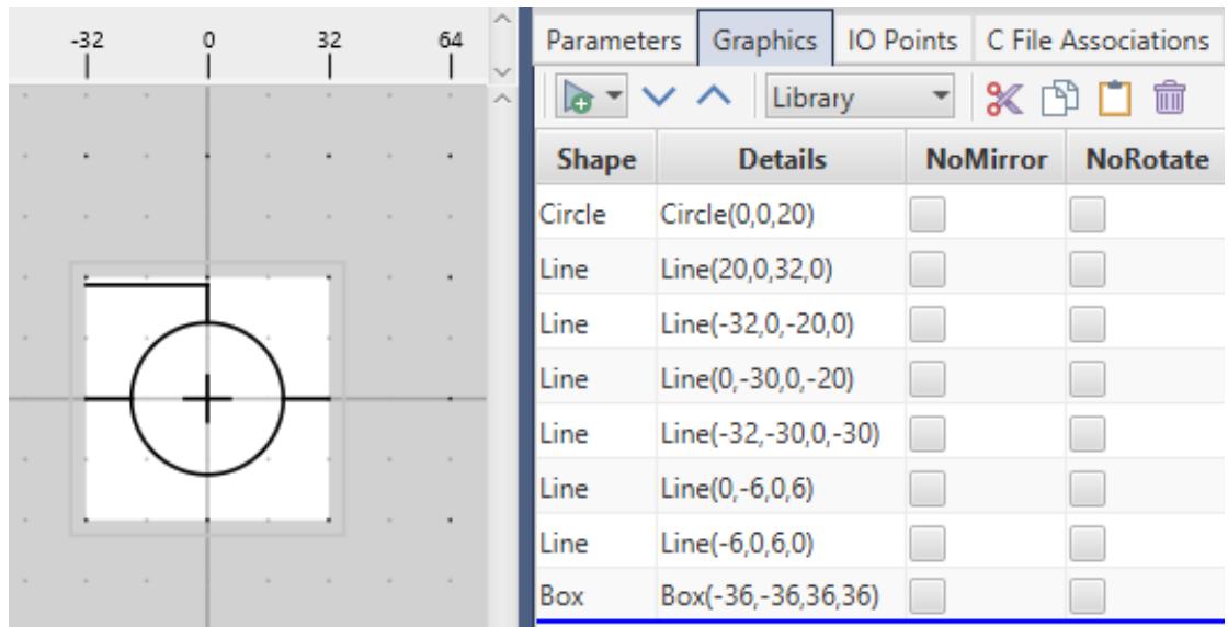
| 1.4.2 Tiny GraphicsThe tiny graphics section is used in RSCAD when the zoom level of a draft circuit is reduced beyond a chosen threshold. These graphics are meant to be a simplified representation of the component with the aim of reducing the computational burden of rendering graphics when a large network is being viewed. Minimal conditional graphics should be used. Use of text is discouraged and black should be the only graphic colour used. An example is shown in Figure 1.15. | |
|  | |
| Figure 1.15: Tiny Graphics Example | |
| # 1.4.3 Library Graphics | |
| 1.4.3 Library GraphicsThe library graphics are the graphics displayed in the library. This is another simpler representation of the component. Library graphics needs to be drawn in the space provided. Use of conditional graphics is discouraged. An example is shown in Figure 1.16 | |
|  | |
| Figure 1.16: Library Graphics Example | |
| # 1.4.4 Loadflow Graphics | |
| 1.4.4 Loadflow GraphicsThis section is applicable for power system components only. Control components do not participate in the loadflow so this section will remain blank for control components. | |
| # 1.5 ADD THE IO POINTS | |
| In this example some of the IO points are conditional. | |
| Select the 'IO Points' tab. | |
| Add 3 nodes using the 'Draw Node' button from the toolbar, Clicking twice on the button will allow several nodes to be drawn successively. Place two of the nodes at the first 2 inputs, place the third at the output of the component. Node details can be modified by selecting each node and editing the information box that appears below the graphics window. See Figure 1.17. | |
| 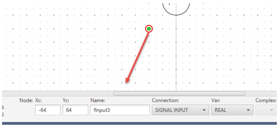 | |
| Figure 1.17: Adding Node Information | |
| The information for the IO nodes are listed below. | |
| # IO point flnput1 | |
| <table><tr><td>Name</td><td>flnput1</td></tr><tr><td>Type</td><td>SIGNAL INPUT</td></tr><tr><td>Data Type</td><td>REAL</td></tr></table> | |
| # IO point flnput2 | |
| <table><tr><td>Name</td><td>flnput2</td></tr><tr><td>Type</td><td>SIGNAL INPUT</td></tr><tr><td>Data Type</td><td>REAL</td></tr></table> | |
| # IO point fOutput | |
| <table><tr><td>Name</td><td>fOutput</td></tr><tr><td>Type</td><td>SIGNAL OUTPUT</td></tr><tr><td>Data Type</td><td>REAL</td></tr></table> | |
| Inside the IO tab, create an 'If' condition and enter 'numInputs $= = 3^{\prime}$ as the condition. | |
| Select the condition 'If numInputs $= = 3^{\prime}$ to ensure the insertion point is inside the condition and add the flnput3 IO point (input to sign3). | |
| 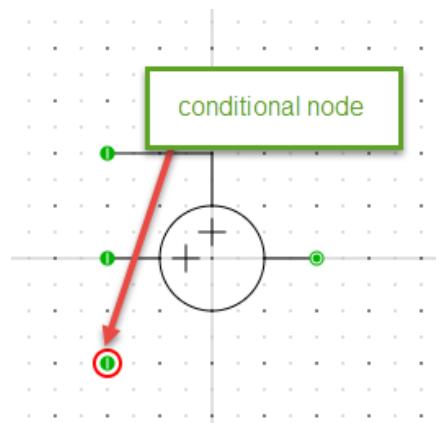 | |
| Figure 1.18: Adding Conditional Graphics | |
| # IO point fInput3 | |
| <table><tr><td>Name</td><td>flnput3</td></tr><tr><td>Type</td><td>SIGNAL INPUT</td></tr><tr><td>Data Type</td><td>REAL</td></tr></table> | |
| The IO tab should now appear as shown in Figure 1.19. | |
| 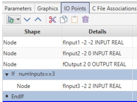 | |
| Figure 1.19: Creating Conditions in IO Points Tab | |
| # 1.6 ADDING THE MODEL CODE | |
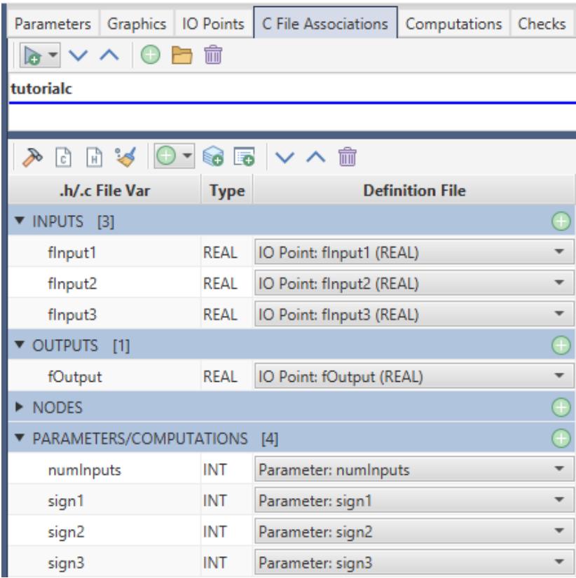
| - Select the 'C File Associations' tab.- Select the + icon to Add New Association.- Enter a model name such as 'tutorialc'- The associations should appear similar to Figure 1.20. | |
|  | |
| Figure 1.20: Adding a New Association | |
| - The input and output points appear under the 'INPUTS' and 'OUTPUTS' sections and not the 'NODES' section. This is a controls component and the NODES section is reserved for power system component electrical type nodes.- The next step is writing the c-code which defines the behaviour of the component. Select the $\square$ icon to begin editing the .c file.Simple 'c' code to add two inputs together and produce an output might look something like the following: | |
| CODE: fOutput $=$ fInputl $^+$ fInput2; | |
| - Type the c-code listed in Section 1.7 into tutorialc.c then push the compile icon in the C File Association tab, to compile the code. If the compile is successful, the component is ready to be included in a Draft circuit.- Ensure that the CBuilder component is saved.- Draft has an internal memory of the components used during a draft session. If a component icon is modified while Draft is open, the icons must be refreshed. Select the $\square$ icon from the library toolbar to refresh components. | |
| # 1.7 SAMPLE 'C' CODE FOR THE MULTIPLE INPUT ADDER | |
| Note: The code should not be copy pasted due to encoding issue. The user should write the code in their editor. | |
| # Code is shown below: | |
| include "tutorialc.h" | |
| STATIC: // use the mult variables to keep track of sign of input int multl; int mult2; int mult3; | |
| # RAM: | |
| // the parameters signl, sign2 and sign3 are toggles where // $0 = =$ plus and $\mathrm{\bf 1} = =$ minus // use the mult variables to keep track of sign of input if $\mathrm{\bf sign1} = =\mathrm{\bf 1}$ | |
| mult1 = - 1; else mult1 = 1; if (sign2 == 1) mult2 = - 1; else mult2 = 1; if (sign3 == 1) mult3 = - 1; else mult3 = 1; | |
| CODE: | |
| if (numInputs > 2) fOutput = (mult1 * fInput1) + (mult2 * fInput2) + (mult3 * fInput3); else fOutput = (mult1 * fInput1) + (mult2 * fInput2); | |
| # 2 INTEGRATOR | |
| # 2.1 INTRODUCTION | |
| The integrator reads in one real input, integrates the input with a user specified time- constant (T) and writes one output. The basic equations, based on trapezoidal rule of integration with a simulation time- step of $\Delta t$ , are used to compute the integral of the input as shown in Equation 2- 1, Equation 2- 2, Equation 2- 3, and Equation 2- 4. | |
| 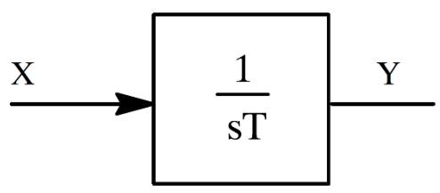 | |
| Figure 2.1: Basic Integral | |
| $$ | |
| Y(t) = \frac{1}{T}\int X(t)dt | |
| $$ | |
| Equation 2- 1 | |
| $$ | |
| Y(t) = \frac{1}{T}\int_{t - \Delta t}^{t}X(t)dt + Y(t - \Delta t) | |
| $$ | |
| Equation 2- 2 | |
| $$ | |
| Y(t) = \frac{1}{T}\left\{\frac{\Delta t*[X(t - \Delta t) + x(t)]}{2}\right\} +Y(t - \Delta t) | |
| $$ | |
| Equation 2- 3 | |
| $$ | |
| Y(t) = \frac{\Delta t}{2T}\{X(t - \Delta t) + x(t)\} +Y(t - \Delta t) | |
| $$ | |
| Equation 2- 4 | |
| # Data Preparation: | |
| Initialize Xold $= 0.0$ Initialize Yold $= 0.0$ Compute $k = dt / (2T)$ | |
| # Algorithm: | |
| Read X; $\mathsf{Y} = \mathsf{K}^{\ast}(\mathsf{Xold} + \mathsf{X}) + \mathsf{Yold};$ Write Y; | |
| # 2.2 DRAW GRAPHICS AND ADD PARAMETERS | |
| Draw an icon that looks similar to Figure 2.2. | |
| 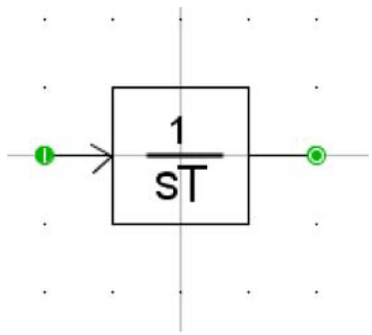 | |
| Figure 2.2: Integrator Component Icon | |
| The component icon for the integrator includes two I/O points. One signal input named input and one signal output named output, both are real.- | |
| Add a parameter 'T' to specify the time constant (type REAL). | |
| # 2.3 ADDING THE MODEL CODE | |
| Select the 'C File Associations' tab.- Select the "Add new Association" which is a plus sign on a green circle.- Enter the model name as "integrate".- Select the "Edit C File" to write the code. | |
| Input and Output points (listed under the IO Points tab) and user defined parameters (listed under the Parameters tab) are automatically associated with the model and placed in the .h file. Left clicking the "View .h file" button opens the .h file in an editor. A model that includes one input, one output and a parameter would have the following lines in the .h file: | |
| INPUTS: double input; OUTPUTS: double output; | |
| # PARAMETERS: | |
| double T; | |
| # 2.4 SAMPLE 'C' CODE FOR AN INTEGRATOR | |
| include "integrate.h" | |
| # STATIC: | |
| /* * Variables declared here may be used in both the */ /* RAM: and CODE: sections below. */ /* double dt; double input_old, output_old, K; /* - E n d o f S T A T I C : S e c t i o n - */ | |
| # RAM: | |
| /* Place C code here which computes constants */ /* required for the CODE: section below. The C */ /* code here is executed once, prior to the start */ /* of the simulation case. */ /* dt= getTimeStep(); input_old = 0.0; output_old = 0.0; K = dt / (2.0 * T); */ | |
| /* - - - - E n d o f R A M : S e c t i o n - - - - */ | |
| CODE: /* */ /* Place C code here which runs on the RTDS. The */ /* code below is entered once each simulation */ /* step. */ /* output = (input + input_old) * K + output_old; input_old = input; output_old = output; | |
| # 2.5 ADD A RESET INPUT TO THE INTEGRATOR | |
| Add shapes to the icon to include a reset input. | |
| 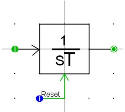 | |
| Figure 2.3: Adding Reset Input to Integrator | |
| - Add an integer I/O point named reset to the reset input.- Update the association to include the new I/O point.- Modify the 'C' code to reset the integrator when a value other than 0 is applied to the reset input.- Recompile the new code.- Save the new icon. | |
| CODE: | |
| if (reset != 0) { | |
| # Builder Tutorial: Integrator | |
| output $= 0$ input_old $= 0$ output_old $= 0$ } else { output $=$ input $^+$ input_old) \* K $^+$ output_old; input_old $=$ input; output_old $=$ output; } | |
| Draft has an internal memory of the components used during a draft session. If a component icon is modified while Draft is open, the icons must be refreshed. Select the $\odot$ icon from the Draft toolbar to refresh components. | |
| Note: Compile the model. The component is now ready. Make sure to save the file. User can load it in RSCAD and test out the component. In order to load the component in RSCAD, right click on a an empty spot in draft, and select Add Component > User > load the definition file. | |
| # 3 VARIABLE CAPACITOR | |
| # 3.1 INTRODUCTION | |
| This component will be modeled as a power system component in CBuilder. | |
| Control system components interact with other components using control type input and output signals and do not interact directly with the solution of the power system network. Power system components, on the other hand, need to interact directly with the solution of the power system network. The interface is usually made by specifying an impedance at the nodes to which the component is connected and by providing current injections into those nodes. | |
|  | |
| Figure 3.1: Current Injection | |
| The network solution expects to receive current injection values from power system components well before the end of the simulation time- step so that there is enough time remaining in the time- step to compute the new node voltages. To accommodate this, the CODE: section for power system components is divided into two portions Begin- T0 and T0- T2. | |
| The first portion, referred to as Begin- T0, is used to execute the statements required to compute current injections which the component injects into the nodes to which it is connected. Once the current injections are ready, the executable code is suspended until all of the other power system models have completed their current injection calculations. At this point the current injections from all of the power system models allocated to the RTDS rack are sent to the processor/core dedicated to solving the power system network. Upon completion of this T0 transfer, executable code for the components who participated in T0 continues. The remaining portion of the executable code, referred to as T0- T2 may be used to solve portions of the algorithm that are not needed to compute the current injections, for preparing variables that are written out for monitoring and preparing for the next time- step. | |
| Once the second portion of code is completed the executable code is again suspended until all of the variables transferred during the T2 communication interval have been transferred between processors. Control type variables, monitored variables and node voltages are exchanged during the T2 communication interval. The node voltages are computed by the processor allocated to the network solution and transferred to other processors in the rack. As such, new node voltage data is available once the processors are restarted for the next simulation time- step. | |
| # 3.2 CAPACITOR | |
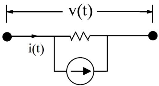
| Application of the trapezoidal rule of integration to the basic capacitor equation is used for the numerical solution of the capacitor. | |
| 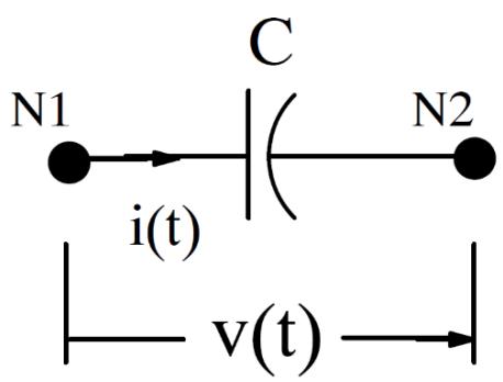 | |
| Figure 3.2: Simple Capacitor | |
| $$ | |
| V(t) = V_{N1}(t) - V_{N2}(t) | |
| $$ | |
| $$ | |
| i(t) = C*\frac{dV(t)}{dt} | |
| $$ | |
| $$ | |
| V(t) = \frac{1}{C}\int i(t)dt | |
| $$ | |
| Equation 3- 1 | |
| Equation 3- 2 | |
| Equation 3- 3 | |
| $$ | |
| V(t) = \frac{1}{C}\int_{t - \Delta t}^{t}i(t)dt + V(t - \Delta t) | |
| $$ | |
| Equation 3- 4 | |
| Applying trapezoidal rule of integration results in Equation 3- 5. | |
| $$ | |
| i(t) = \frac{2C}{\Delta t} *V(t) - \frac{2C}{\Delta t} *V(t - \Delta t) - i(t - \Delta t) | |
| $$ | |
| Equation 3- 5 | |
| 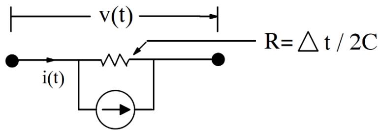 | |
| Figure 3.3: IH: Current Injection | |
| Define: | |
| $$ | |
| IH(t) = -\frac{2C}{\Delta t} *V(t - \Delta t) - i(t - \Delta t) | |
| $$ | |
| $$ | |
| i(t) = \frac{2C}{\Delta t} *V(t) + IH(t) | |
| $$ | |
| Equation 3- 6 | |
| Equation 3- 7 | |
| # 3.3 DRAW GRAPHICS AND ADD PARAMETERS | |
| Draw a capacitor icon similar to that shown in Figure 3.4. | |
| 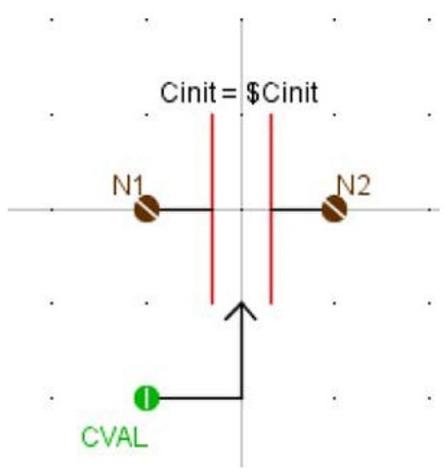 | |
| Figure 3.4: Capacitor Icon | |
| The component icon for the variable capacitor includes two power system nodes and one signal input as shown in Figure 3.4. The signal input 'CVAL' is used to read in variable capacitance values. | |
| Add a parameter 'Cinit' to specify the initial value of capacitance. | |
| A power system node is created by creating an I/O Point/Node and selecting "PSYS Node" as the connection type. | |
| # 3.4 ADDINGTHEMODELCODE | |
| Select the 'C File Associations' tab.- Select the icon to Add New Association.Creating the C File Associations for the component automatically generates the following associations: | |
| INPUTS: CVAL, capacitance value signal input | |
| NODES:N1,N2 power system nodes | |
| PARAMETERS:Cinit, initial value of capacitance | |
| In addition to those listed above, the following additional associations need to be made: | |
| GVALUES: A conductance value (1/R) that the component places between the nodes to which it is connected. Recall, that the representation of the capacitor requires a resistor equal to $\Delta t / (2C)$ to be placed between the nodes to which the component is connected. The equivalent conductance is equal to $1 / R = 2C / \Delta t$ . To add the GVALUE association select the Add Variable to .h File "+" button from the C File Associations Tab and select New GValue. Edit new gvalue window will appear at the right hand side when the gvalue line is selected. Type will be Real and enter the variable name to which the conductance value will be assigned in the .c code. | |
| 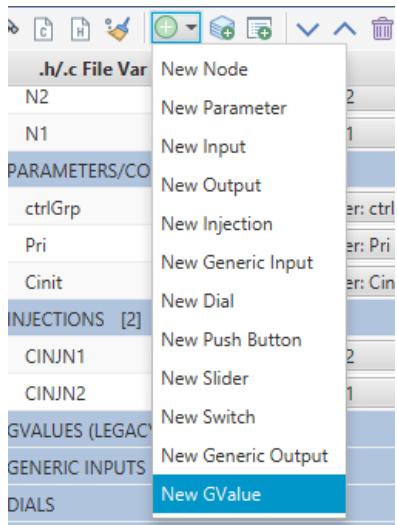 | |
| Figure 3.5: Adding Gvalues to Power System Model | |
| INJECTIONS: The capacitance model injects current into node2 and out of node1. To add an injection, click the + on the injections section. Type: REAL. Enter the name for the current injection variable (CINJN1). Select the down arrow icon for the | |
| CINJN1 variable and select Node N1. Add another current injection variable (CINJN2) and associate it with Node N2. | |
| <table><tr><td colspan="3">INJECTIONS [2]</td></tr><tr><td>CINJN1</td><td>REAL</td><td>Node: N1</td></tr><tr><td>CINJN2</td><td>REAL</td><td>Node: N2</td></tr></table> | |
| - Selecting File->Save causes the newly added GVALUES and INJECTIONS variables to be written to the .h file so they can be accessed in the .c file. | |
| - Write the 'c' code. Select the icon to edit the .c file. | |
| Basic Algorithm: | |
| Read 2 node voltages v1(t), v2(t) Compute $\mathsf{V}(\mathsf{t}) = \mathsf{v}1(\mathsf{t}) - \mathsf{v}2(\mathsf{t})$ Compute branch current: $\mathsf{i}(\mathsf{t}) = 2\mathsf{C} / \Delta \mathsf{t}^{*}\mathsf{V} + \mathsf{IH}(\mathsf{t} - \mathsf{dt})$ note: IH(t) from previous time- step Read Capacitance Value Compute $\mathtt{Gc} = 2\mathtt{C} / \Delta \mathtt{t}$ Set new Gc value for network solution Compute Injection Current: $\mathsf{IH}(\mathsf{t}) = - 2\mathsf{C} / \Delta \mathsf{t}^{*}\mathsf{V} - \mathsf{i}(\mathsf{t})$ Set injection current for node1 and node2 | |
| The RAM section initializes the history term current IH(t- dt) to 0.0 and computes the constant 1/Δt for use in the CODE: section. | |
| Static: double dt, invdt, Ih, Gcap, Vbra, ib; | |
| RAM: dt $=$ getTime- step(); invdt $=$ 1.0/dt; $\mathbb{I}\mathfrak{h} = \mathbb{0},\mathbb{0}$ . Gcap $=$ 2.0 \* Cinit \* 1.0e- 6 \* invdt; | |
| The CODE: section computes the branch current for the capacitor, the new conductance for the capacitance and the current injections into the nodes between which the component is connected. All of the code is assigned to the BEGIN_TO portion since it is required to compute the injection currents. The capacitance value is read in as micro- farads (i.e. 1.0 is interpreted as 1.0e- 6 farads) so the CVAL variable must be multiplied by 1.0e- 6 before it can be used. | |
| CODE: | |
| BEGIN_T0: | |
| /* Compute branch current */ Vbra = N1 - N2; ib = Gcap * Vbra + Ih; | |
| /* Compute new value of Cfarad */ Gcap = 2.0 * CVAL * 1.0e- 6 * invdt; GCVAL = Gcap; | |
| /* Compute new History Current */ Ih = - Gcap * Vbra - ib; | |
| /* Write current injections into N1, N2 */ /* +ve means current out of node */ CINJN1 = Ih; CINJN2 = - Ih; | |
| # 3.5 ADDING AN OPTIONALLY MONITORED VARIABLE | |
| It is often desirable to permit the user to optionally monitor various internal variables associated with a component. Monitoring of such internal variables may be useful for debugging when the component is part of a larger control circuit. The monitoring may be included without adding additional output points to the component. The following procedure is suggested: | |
| 1. Add a Yes/No Toggle type parameter which permits the user to select whether the current is to be monitored in a new section called "MONITORING". (see 1 of Figure 3.6). | |
| 2. Add a Name type parameter which permits the user to enter a name for the monitored | |
| current. The Name entry can be made conditional on the monitoring being enabled in a new section called "Signal Names" (see 2 of Figure 3.6). | |
| 3. Add a new generic output variable which is active only if the monitoring is enabled in the C File Association. | |
| 4. Add statements to the RTDS C code to assign the branch current to the monitored variable. | |
| 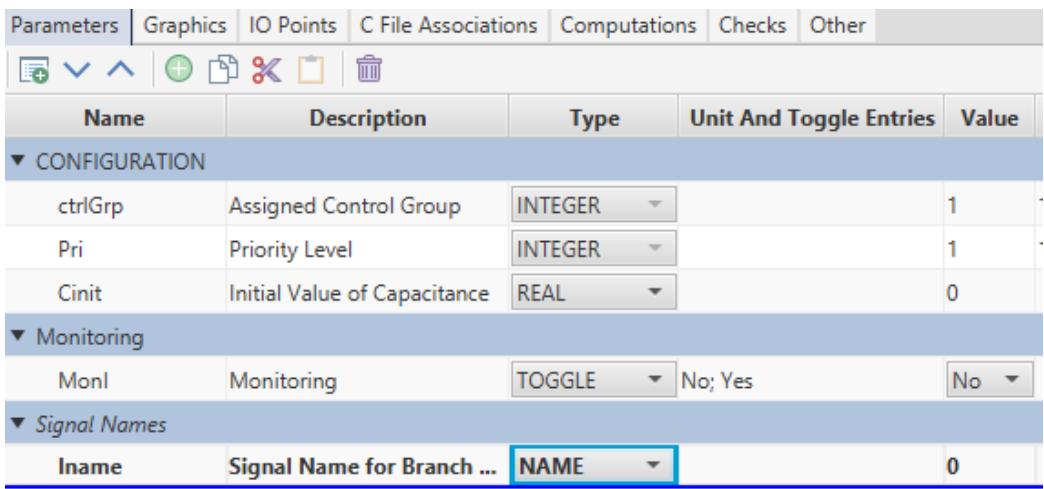 | |
| Figure 3.6 Adding a Monitored Variable in CBuilder | |
| The new parameters Monl and Iname must be added to the .h file. Select the Add New IO Points/Nodes/Parameters/Computations to Association icon from the C File Associations tab to add these new parameters. | |
| 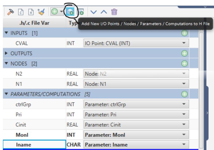 | |
| Figure 3.7: Adding New IO Points to C File Association | |
| To add the monitored variable parameter to the .h file, left click the Add Variable to .h File button under the C File Associations tab. Select create: Generic Outputs from the pulldown menu associated with the Section: field and set Type: to REAL. Enter a variable name (e.g. IMON) to be used for assignment of the monitored variable in the .c file. After selecting OK, the Edit Output menu appears in which additional parameters for the output variable may be specified. | |
| 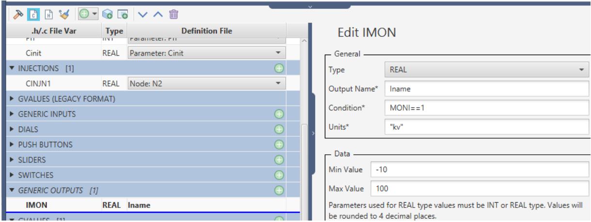 | |
| Figure 3.8: Editing The Generic Output Section | |
| Type: REAL H File VAR: IMON Output Name: iname Group: "Branch Currents" Min Value: - 100.0 Max Value: +100.0 Unit: "kA" Condition: Monl=+1 | |
| Min and Max values are used as the default limits for a meter or plot component assigned to display the signal specified by Output Name. The specified unit name also appears on the meter or plot component in RSCAD/RunTime. | |
| The create: OUTPUTS data line for the monitored output variable appears as: | |
| 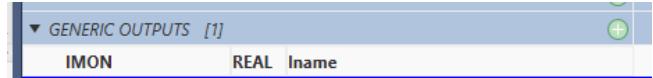 | |
| Figure 3.9: Creating a Generic Output | |
| "1" is the parameter name for .c file.- "2" is the signal name available in RSCAD/RunTime. | |
| The C code statement to write out the monitored variable is as follows: | |
| IMON = ib;- The current monitoring should be assigned in the T0_T2 section of the CODE. | |
| # 4 MULTI-MASS SYSTEM | |
| # 4.1 INTRODUCTION | |
| Representation of the mechanical characteristics of turbine generator units in electromagnetic transients programs is necessary if the interaction between the electrical system and mechanical system is to be studied. In some situations a resonant condition may exist between the electrical system and the mechanical system which can lead to torsional oscillations which stress the mechanical couplings between the various turbines and between the turbine and generator. Perhaps the best documented case of such a resonance was at the Navajo Project, a coal fired generation unit located in northern Arizona, U.S.A. [1]. Data from the Navajo Project was used to develop a first and second benchmark model for torsional oscillations [2],[3]. | |
| This document outlines how the mechanical characteristics of a turbine- generator system may be incorporated into a model for use on the RTDS. Once the equations for the multi- mass system have been developed, the procedure for implementing the corresponding algorithm using the CBuilder feature under RSCAD is documented. | |
| Development of the equations representing the mechanical system follows that presented in Kundar [4]. Firstly, the equations of motion for a single mass rotating about an axis are developed. The analysis is then expanded to account for two masses connected by a shaft and finally generalized to multiple masses. | |
| # 4.2 SINGLE MASS ROTATING ABOUT AND AXIS | |
| # 4.2.1 EQUATIONS OF MOTION REPRESENTING A SINGLE MASS ROTATING ABOUT AN AXIS | |
| 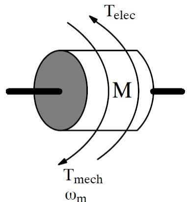 | |
| Figure 4.1: Single Mass Rotating Motion | |
| The basic equation of motion for a rotating mass stems from Newton's Second Law of motion (commonly stated as $F = mA$ ) where the Force is the difference between the mechanical torque applied by a turbine and the electrical torque applied across the air- gap of the generator. Acceleration for the rotating mass is the rate of change of its rotational speed $(\omega_{m})$ . Instead of the mass of the rotating body, the mass' moment of inertia (J) is used. The moment of inertia considers both the rotating body's mass and its distribution around the axis of rotation. | |
| $$ | |
| J\frac{d\omega_{m}}{dt} = T_{m - }T_{e} \tag{[1]} | |
| $$ | |
| J Mass' moment of Inertia in $\mathsf{kg}\cdot \mathsf{m}^2$ $\omega_{m}$ rotational speed of the mass in mech. rad/sec $T_{m}$ Mechanical torque applied by the turbine $(N\cdot m)$ $T_{e}$ Electrical torque applied by the generator $(N\cdot m)$ $(1N = 1kg\cdot m / sec^2)$ | |
| It is important to note that $\omega_{m}$ in [1] above represents the mechanical rotational speed of the machine in rad/sec. It is to be differentiated from the machine's electrical rotational speed. Mechanical speed and electrical speed is the same for a machine with only one pole pair. Machines that have more than a single pole pair will have a slower mechanical rotational speed than one with just one pole pair. | |
| $$ | |
| \omega_{e} = \omega_{m}*n | |
| $$ | |
| By using the per- unit inertia constant, H, which is defined as the mass' kinetic energy in watt- seconds at rated speed, as opposed to the moment of inertia, equation [1] can be expressed in terms of electrical rad/sec. H and J are related as - | |
| $$ | |
| \begin{array}{c}{H = \frac{1}{2}\frac{J\omega_{0m}^2}{VA_{base}}}\\ {J = 2\frac{H}{\omega_{0m}^2} VA_{base}} \end{array} \tag{2} | |
| $$ | |
| $\omega_{0m}^{2}$ rated rotational speed of the mass in mechanical rad/sec. $VA_{base}$ Volt- Amp base for the system | |
| Substituting [2] into [1] yields - | |
| $$ | |
| \frac{2H}{\omega_{0m}^2} VA_{base}\frac{d\omega_m}{dt} = T_m - T_e \tag{3} | |
| $$ | |
| Noting that - | |
| $$ | |
| \begin{array}{c}{\omega_{m} = \omega_{r} = \omega_{pu}}\\ {\omega_{0m} = \omega_{0}}\\ {T_{base} = \frac{VA_{base}}{\omega_{0m}},\frac{T}{T_{base}} = T_{pu}} \end{array} \tag{5} | |
| $$ | |
| $\omega_{r}$ rotational speed of the mass in electrical rad/sec $\omega_{0}$ rated rotational speed of the mass in electrical rad/sec. $T_{base}$ base value of mechanical torque we re- arrange equation [3] such that equations [4] and [5] may be substituted. | |
| $$ | |
| \begin{array}{c}{2H\frac{d}{dt}\left[\frac{\omega_m}{\omega_{0m}}\right] = \frac{T_m - T_e}{VA_{base} / \omega_{0m}}}\\ {2H\frac{d}{dt}\left[\frac{\omega_r}{\omega_0}\right] = \frac{T_m - T_e}{VA_{base} / \omega_{0m}}}\\ {2H\frac{d}{dt}\left[\frac{\omega_r}{\omega_0}\right] = \frac{T_m - T_e}{T_{base}}} \end{array} \tag{8} | |
| $$ | |
| Equation [8] above relates the per- unit applied torque to the per- unit rotational speed of the mass. Implementation of equation [8] into the the RTDS solution algorithm may be done by applying trapezoidal rule to yield - | |
| $$ | |
| 2H\frac{\omega_{pu(t)} - \omega_{pu(t - \Delta t)}}{\Delta t} = \frac{T_{apu(t)} + T_{apu(t - \Delta t)}}{2} \tag{9} | |
| $$ | |
| $T_{a_{pu}}$ per- unit accelerating torque | |
| $$ | |
| T_{a_{pu}} = (T_m - T_e) / T_{base} | |
| $$ | |
| At the beginning of the simulation time- step all of the quantities in [9] listed as functions of $(t - \Delta t)$ are known, as are the constants $2H$ and $\Delta t$ . The most recently computed value of $T_{a_{pu}}$ is used as $T_{a_{pu}(t)}$ . This leaves only $\omega_{pu(t)}$ to be computed. | |
| To demonstrate the action of [9], we can apply a constant 1 per- unit torque with no electrical torque (ie. open circuit conditions for a frictionless generator) and note that the mass' speed linearly increases. Under such conditions the rotating mass reaches 1 per- unit rotational speed after $2H$ seconds. $2H$ is referred to as the mechanical starting time. | |
| 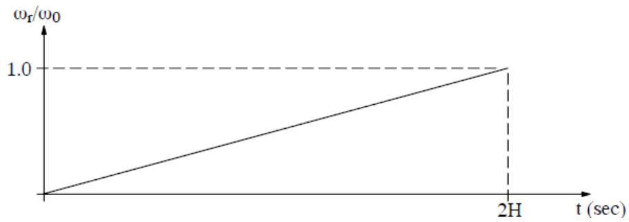 | |
| Figure 4.2: Mechanical Starting Time | |
| # 4.3 DAMPING | |
| In the equations for the rotating mass described above, there was no consideration of damping. Removing the applied torque in the example above results in the mass rotating at $\omega_{pu}$ indefinitely. In [4] a damping term proportional to $\Delta \omega_r$ is introduced. Adding such a term to [8] yields - | |
| $$ | |
| 2H\frac{d}{dt}\left[\frac{\omega_r}{\omega_0}\right] = \frac{T_m - T_e}{T_{base}} -D\Delta \left[\frac{\omega_r}{\omega_0}\right] \tag{[10]} | |
| $$ | |
| Damping proportional to speed deviation (ie. $D\Delta \left[\frac{\omega_r}{\omega_0}\right]$ ) results in an accelerating torque when the speed of the rotating mass is less than the rated speed. Such a representation is reasonable for small perturbations of speed around the rated speed. However, if the mass is to be used as part of a generator - turbine model which is required to have large deviations from synchronous speed, the chosen representation of damping leads to unrealistic behavior. Take for instance the case where the generator is to be started from standstill. At | |
| zero speed the speed deviation is - $1_{pu}$ and according to [10] the mass is subjected to an accelerating torque of $+D_{pu}$ . | |
| A physical interpretation of the damping term proportional to speed deviation is given in the discussion to reference [5]. | |
| A damping term proportional to per- unit speed, representing the friction and windage losses, can be introduced into [8] to obtain [1]. The addition of a speed proportional damping term changes the response of the mass to a constant mechanical torque input as shown in Figure 4.3 (compare with Figure 4.2 which shows the response with no damping term). | |
| $$ | |
| 2H\frac{d}{dt}\left[\frac{\omega_r}{\omega_0}\right] = \frac{T_m - T_e}{T_{base}} -D\left[\frac{\omega_r}{\omega_0}\right] \tag{[11]} | |
| $$ | |
| 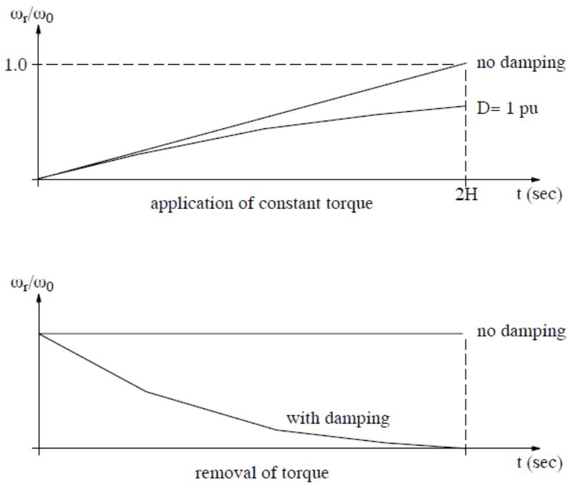 | |
| Figure 4.3: Response With Speed Proportional Damping | |
| Removal of the applied torque, using [11] to represent the rotating mass, results in the mass' rotational speed slowing to 0.0. Note that equation [11] has the same form as a first order lag with a gain of $1 / D$ and a time- constant of $2H / D$ seconds. | |
| 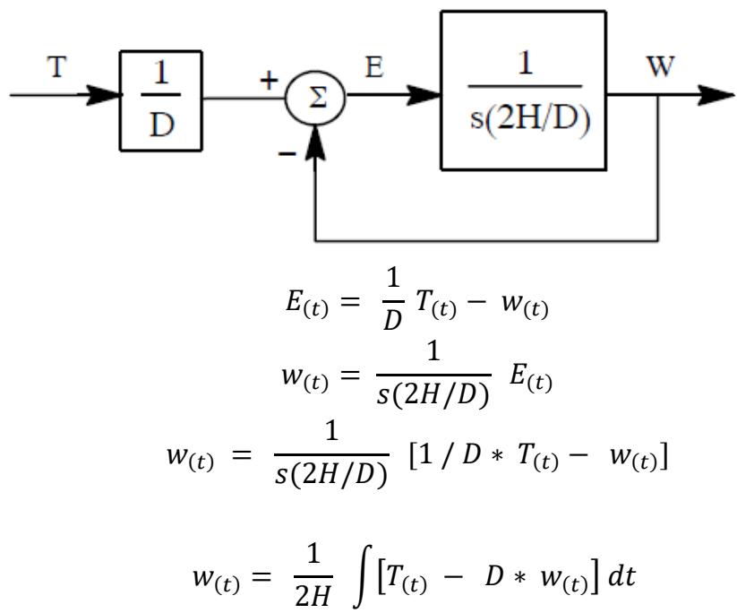 | |
| 1st order lag function with $\text{Gain} = 1 / D$ and time constant $= 2H / D$ . Compare with equation [11] above. | |
| # 4.4 TWO ROTATING MASSES COUPLED BY A SHAFT | |
| 4.4.1 EQUATIONS OF MOTION FOR 2 ROTATING MASSES COUPLED BY A SHAFT | |
|  | |
| Figure 4.4: Two Rotating Masses | |
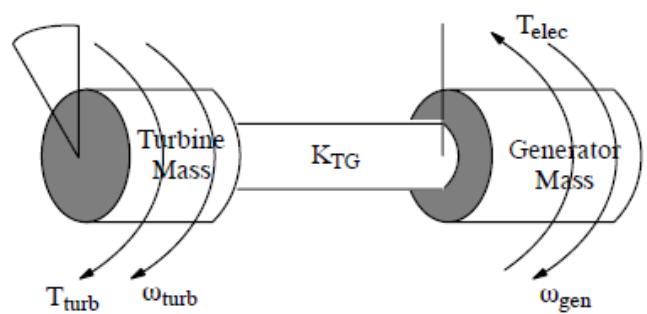
| The equations developed above are now extended to two masses coupled by a shaft. One mass represents a turbine and the other the rotating mass of the generator. The mass of the shaft itself is lumped proportionally into the rotating mass' inertia constants. The shaft connecting the generator mass to the turbine mass is considered as a torsional spring. Torque transferred across the shaft between the turbine and the generator results in | |
| twisting of the shaft. The amount of twist depends on the torque transferred across the shaft and on the torsional strength of the material comprising the shaft. | |
| $$ | |
| T = K\theta_{m} \tag{12} | |
| $$ | |
| T Torque transferred across the shaft $(N_{1}m)$ $\theta_{m}$ Mechanical angle of twist across the shaft (rad) K Shaft Stiffness $(N_{1}m / rad)$ | |
| The shaft stiffness constant $(K)$ defines the torque required to create an angular twist of 1 radian across the shaft. Values of K are typically very large since the torque, in N/m, required to twist a large turbo generator shaft by 1 radian (\~57 degrees) is significant. In order to use [12] with [11] developed above, equation [12] needs to be converted so as to relate per- unit torque to per- unit angle. Using the base values for mechanical angle and torque as shown below - | |
| $$ | |
| \begin{array}{r}\theta_{m_{base}} = \omega_{0m}\\ T_{base} = \frac{VA_{base}}{\omega_{0m}} \end{array} | |
| $$ | |
| the base shaft stiffness may be computed as - | |
| $$ | |
| K_{base} = \frac{VA_{base}}{\omega_{0m}} | |
| $$ | |
| $\omega_{0m}$ rated rotational speed of the mass in mech. rad/sec. | |
| The torque applied by the shaft to the masses to which it is attached is given by - | |
| $$ | |
| \begin{array}{l}{T_{T G} = K_{T G}(\theta_{T} - \theta_{G})}\\ {}\\ {T\qquad \mathrm{in~pu~if~}K_{T G}\theta \mathrm{~in~pu~}} \end{array} | |
| $$ | |
| The equations of motion for the two rotating masses can now be written - | |
| Generator Mass | |
| Turbine Mass | |
| Shaft Angle | |
| $$ | |
| \begin{array}{c}{2H\frac{dw_{gen}}{dt} = T_{turb} - T_e - D_{gen}\omega_{gen}}\\ {2H\frac{dw_{gen}}{dt} = T_{turb} - D_{turb}\omega_{turb}}\\ {\theta_T - \theta_G = \frac{T_{turb} - T_e}{K_{TG}}} \end{array} \tag{13} | |
| $$ | |
| All quantities in per- unit | |
| Equations [13] and [14] can be solved numerically using the trapezoidal rule as - | |
| $$ | |
| 2H\frac{\omega(t) - \omega(t - \Delta t)}{\Delta_t} +D\frac{\omega(t) - \omega(t - \Delta t)}{2} +K\frac{\theta(t) + \theta(t - \Delta t)}{2} = \frac{T(t) + T(t - \Delta t)}{2} \tag{16} | |
| $$ | |
| All of the history terms (ie. those at $t - \Delta t$ ) are known at the start of a new time- step. $2H$ , $D$ , $K$ and $\Delta t$ are constants and the new value of applied torque $T(t)$ is assumed to be known. The values $\omega (t)$ and $\theta (t)$ are unknown at the beginning of the time- step. Using the relation (17a) and applying trapezoidal rule an expression for $\theta (t)$ can be derived in terms of $\omega (t)$ . | |
| $$ | |
| \begin{array}{c}\frac{d\theta}{dt} = \omega \\ \displaystyle \frac{\theta(t) - \theta(t - \Delta t)}{dt} = \frac{\omega(t) + \omega(t - \Delta t)}{2}\\ \displaystyle \theta (t) = \frac{\Delta t}{2} [\omega (t) + \omega (t - \Delta t] + \theta (t - \Delta t) \end{array} \tag{17b} | |
| $$ | |
| Equation [17c] can be substituted into [16] to eliminate the $\theta (t)$ term and leave $\omega (t)$ as the only unknown. | |
| $$ | |
| \omega (t)\left[\frac{2}{\Delta t} 2H + D + \frac{\Delta t}{2} K\right] = | |
| $$ | |
| $$ | |
| T(t) + T(t - \Delta t) + \omega (t - \Delta t)\left[\frac{2}{\Delta t} 2H - D - \frac{\Delta t}{2} K\right] - 2K\theta (t - \Delta t) \tag{18} | |
| $$ | |
| $$ | |
| \begin{array}{c}{d e f i n e A = \left[\frac{2}{\Delta_{t}} 2H + D + \frac{\Delta_{t}}{2} K\right]}\\ {B = \left[\frac{2}{\Delta_{t}} 2H - D - \frac{\Delta_{t}}{2} K\right]} \end{array} \tag{19} | |
| $$ | |
| solving for $\omega (t)$ in [18] substituting $A$ and $B$ as defined above yields - | |
| $$ | |
| \omega (t) = A^{-1}[T(t) + T(t - \Delta t) + \omega (t - \Delta t)[B] - 2K\theta (t - \Delta t)] \tag{20} | |
| $$ | |
| Equation [20] is solved for each mass substituting in the appropriate parameters for $H$ , $D$ and $T$ . | |
| It is worth noting that the constants defined in [19] include terms which are multiplied by $2 / \Delta t$ and $\Delta t / 2$ . For a typical simulation time- step of $50 \mu s$ these multiplying factors vary by ten orders of magnitude. Given typical values for $H$ and $K$ the constants can be computed as - | |
| $$ | |
| \begin{array}{l}\frac{2}{\Delta t} *2H = \frac{2.0}{50e^{-6}} *2*0.8688 = 69,504.0\\ \displaystyle \frac{\Delta t}{2} *K = \frac{50e^{-6}}{2.0} *14042.92 = 0.3511 \end{array} | |
| $$ | |
| Even with the typically large difference in magnitude between $H$ and $K$ the elements comprising constants $A$ and $B$ are still different by five orders of magnitude. As for the damping factor $(D)$ which is also required to compute $A$ and $B$ , there is little in the way of typical data available in the literature. In many cases the damping is set to zero. | |
| # 4.5 MULTI-MASS MODEL USING MATRIX FORMULATION | |
| Representation of n masses coupled by shaft segments is straight forward. By arranging the equations developed for 2 masses in matrix form, the solution can be generalized to any number of masses. For the present model, matrix sizes are dimensioned to permit eight turbine masses, one generator mass and two rotating exciter masses for a total of 11 coupled masses. | |
| 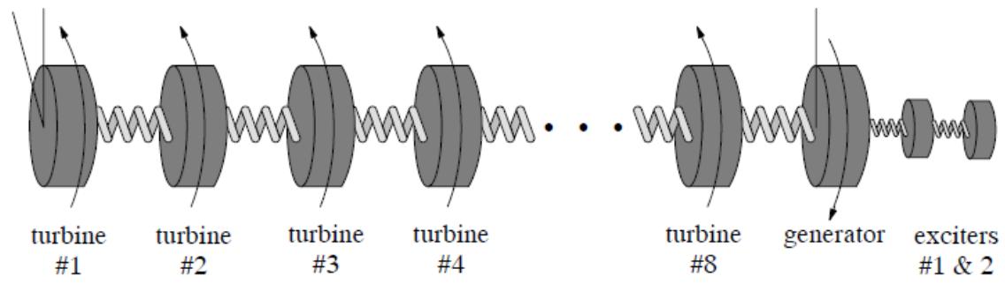 | |
| Figure 4.5: Multi Mass | |
| Equation [20] re- written in matrix form is - | |
| $$ | |
| [\omega_{n}(t)] = [A^{-1}][[T_{n}(t - \Delta t)] + [\omega_{n}(t - \Delta t)][B] - [2K][\theta_{n}(t - \Delta t)] \tag{21} | |
| $$ | |
| where - | |
| $n$ mass index 1. .. number of masses $[\omega_{n}(t)]$ newly computed speed of mass n $[A^{- 1}]$ inverse of tri- diagonal matrix A (full matrix) $T_{n}(t)$ latest value of torque applied to mass n | |
| $T_{n}(t - \Delta t)$ previous value of torque applied to mass n $[\omega_{n}(t)]$ previously computed value of speed of mass n [B] tri- diagonal matrix of B constants [2K] tri- diagonal matrix of $2*K$ spring constants $[\theta_{n}(t - \Delta t)]$ previous value of mass angle [D]: tri- diagonal damping coefficient matrix used in the calculation of the $A$ and $B$ matrices. | |
| The damping matrix includes both terms for the diagonal and off diagonal elements. Diagonal elements represent the self- damping factors (friction, windage) described above. Off- diagonal terms represent the damping due to the twisting of the shaft. Under transient conditions, when a varying torque is applied across the shaft segments, the back and forth twisting of the shaft results in heating and hence some damping. Data for this mutual damping is often not available. Note that the mutual damping is across a shaft segment so that only the $n - 1$ , $n$ and $n + 1$ elements of the damping matrix have non- zero terms. | |
| $$ | |
| D = \left[ \begin{array}{cccc}X_{11} & X_{12} & 0 & 0\\ X_{21} & X_{22} & X_{23} & 0\\ 0 & X_{32} & X_{33} & X_{34}\\ 0 & 0 & X_{43} & X_{44} \end{array} \right] \tag{22} | |
| $$ | |
| Damping Matrix form for 4 mass system | |
| # 4.6 MULTI-MASSMODELALGORITHM | |
| The algorithm for the multi- mass model is based on the solution of equation [21] above. The dimension of matrices and column vectors required for the solution is determined by the number of masses that constitute the system under study. Solution of [21] requires that mechanical torque applied to the turbines, electrical torque from the generator, a number of constants and information from the previous time- step are known. | |
| Mechanical torque to each turbine is provided as input to the multimass model from a separate component which models the speed control and torque production. Electrical torque is provided as output from the synchronous machine model or from the induction motor model and passed to the multimass model. User entered data, $H_{n},K_{n},D_{n}$ and simulation time- step are used to compute constants $A1,B$ and $[2K]$ | |
| Solution of [21] solves for mass rotational speeds from which mass angles and shaft torques can be computed. These quantities are provided as output from the multimass model. | |
| A mechanism is provided to lock all of the modelled mass speeds to a specified speed (often synchronous speed). A lock/free switch can be created in RSCAD/RunTime as part of the model, or the user can provide the lock/free signal input from an external signal. When in lock mode, all mass rotational speeds are set equal to the specified speed. Lock mode is often used to temporarily bypass the turbine dynamics during initialization of the power system to which the multimass system is connected. | |
| It is also possible operate the multimass model so as to lump all of the masses into a single rotating mass. In this way the shaft dynamics can be removed. A single/multi switch can be created in RSCAD/RunTime as part of the model, or the user can specify that the single/multi signal come from an external source. When in single mode, the torques applied to all of the turbine masses are added to form a single mechanical torque input. The equivalent mass' inertia constant is equal to the sum of all modelled masses. The sum of all the self damping terms is used for the damping. | |
| # 4.7 MODEL DEVELOPMENT USING C-BUILDER | |
| Development of the multi- mass model requires the following steps - | |
| # 4.7.1CONCEPTUAL LAYOUT OF THE NEW COMPONENT | |
| a. Which inputs should be connected using wires | |
| b. Which outputs should be connected using wires | |
| c. appearance of the component icon | |
| d. options which change appearance of icon | |
| e. What data is required to prepare the constants | |
| f. How to group related data fields | |
| g. What monitoring options should be available | |
| h. control system or power system component type | |
| # 4.7.2 COMPONENT ICON CREATION IN C-BUILDER (GRAPHICS & NODES) | |
| a. Define component as a Control system typecomponent | |
| b. locate and place all of the input / output points and add associated logic blocks | |
| c. Draw component icon portions which do not require conditional logic. | |
| d. Draw component icon portions for each option which changes the component's appearance. | |
| # 4.7.3 DEFINE USER SUPPLIED DATA MENUS (PARAMETERS) | |
| a. Add all of the data sections defined under I(f) above. | |
| b. Add logic to parameters so the parameter entry fields are visible only when the corresponding options are selected. | |
| # 4.7.4 WRITE DATA PREPARATION PORTION OF THE 'C' PROGRAM | |
| a. Create C File and Declare required variables | |
| b. Compute constants required for the executable code | |
| c. Optionally write critical data to the .map file | |
| # 4.7.5 WRITE 'C' CODE TO IMPLEMENT THE ALGORITHM | |
| a. Declare required variables | |
| b. Create variables for named output signals | |
| c. Create variables for named input signals | |
| # 4.7.6 TEST NEWLY DEVELOPED MODEL | |
| a. Check data preparation to ensure constants are computed correctly. | |
| b. Run simulation cases to confirm basic operation | |
| c. Run simulation cases to verify against benchmark cases | |
| # 4.7.7 CONCEPTUAL LAYOUT OF THE NEW COMPONENT | |
| a. Torque inputs to each turbine section and the generator $(Te)$ will be connected to input points. The user will thus be able to interconnect the governor/torque production model to the multimass model via wires. The synchronous generator model's Te output signal can also be connected to the multimass model via a wire component. | |
| b. The synchronous generator model requires the generator mass speed signal as an input. Note that the speed signal may change very little from simulation time-step to time-step. Within the GPC processor, computations are done using double (64 bit) precision. However, when the data is sent from the multimass model to the generator model over the rack backplane, the speed signal is converted to a single precision number. Rather than sending the speed signal directly from the multimass to the machine model, a delta-omega (ie. change from synchronous speed) signal is sent instead. | |
| Input and output points for the multimass model are shown in Figure 4.6. | |
| 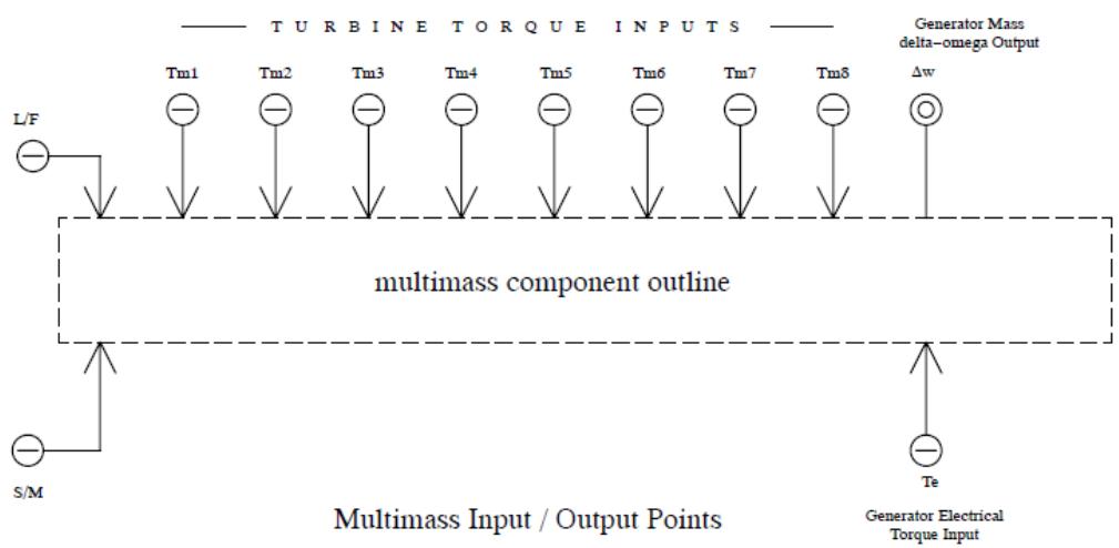 | |
| Figure 4.6: Input and Output Points | |
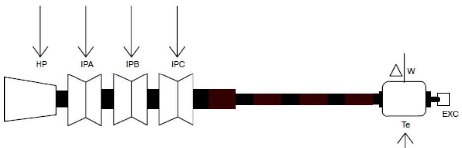
| c. The component's appearance is shown in Figure 4.7. Each of the turbine torque inputs connects to an icon representing a single turbine mass. Electrical torque is connected as an input to an icon representing the rotating portion of the generator. A change from synchronous speed signal for the generator mass is available as an output. At synchronous speed this signal is equal to 0.0. Two exciter masses are connected on the right side of the generator mass. | |
| 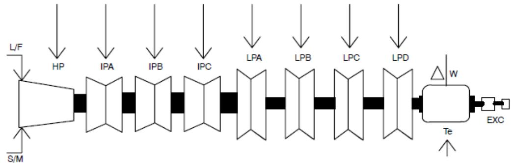 | |
| Figure 4.7: Multimass Component Appearance | |
| d. There are a number of options which may be set by the user which require the appearance of the component icon to change - | |
| Number of turbine masses (1- 8) Number of exciter masses (0- 2) Lock/Free switch input mode Single/Multi switch input mode | |
| The generator mass and HP turbine mass are always drawn. If the number of turbines is set less than 8, then unused turbine icons are replaced by extending the shaft between the generator and last turbine. Exciter masses are drawn only if selected. | |
|  | |
| Figure 4.8: Extended Shaft Between the Generator and Turbine | |
| Multi- Mass component icon with 4 turbine masses, 1 exciter mass and switch inputs created as part of the model. | |
| e. The following data must be supplied by the user before the constants required for the algorithm can be computed - | |
| $H$ Inertia Constant for each mass (MW sec / MVA) $K$ Spring Constant for each shaft (in pu) $D_{s}$ Self Damping for each mass (in pu) $D_{m}$ Mutual Damping for each shaft section (in pu) | |
| Logic is included as part of the component so that only the data required for the number of selected turbines needs to be entered. Data items not required for the selected configuration appear grey in the menus and cannot be selected for input. | |
| f. The following data tabs are defined for the multi-mass component - | |
| CONFIGURATION Basic configuration options INERTIA CONSTANTS $H$ values for each mass SHAFT SPRING CONSTANTS $K$ values for each shaft section SELF DAMPING $D_{s}$ values for each mass MUTUAL DAMPING $D_{m}$ values for each shaft section MONITORING OPTION TABS see below | |
| g. The user is able to select the following items for monitoring. | |
| These are named variables and as such there is no wire protruding from the component icon for any of these outputs. | |
| Mass Speed Mass Angle with respect to the generator Shaft Torque | |
| Tabs are included in the component icon to facilitate selection of the signals to be monitored and the name assigned to each monitored variable. Logic is included as part of the component to permit selection of only those variables which are computed for the specified configuration. | |
| h. C-Builder requires that the user specify whether the component is a power system or control system type component. Power system components connect to power system nodes as defined by node icons in RSCAD/Draft and often contribute current injections into those nodes to which the component is connected. Control system components do not connect to power system nodes and are not able to supply current injections into the power system network. | |
| The GPC processor to which a control system component is allocated automatically becomes a control system processor for the simulation case and only other control system components maybe allocated to that processor. It is not possible to allocate both control system and power system components to the same GPC processor. | |
| # 4.7.8 COMPONENT ICON CREATION IN C-BUILDER | |
| The C- Builder Users Manual should be consulted for additional details on defining the component icon. Information provided here outlines the major steps required to complete the icon associated with the multi- mass model. | |
| a. Define the Component as a Control System Component | |
| When a new component is created the user is prompted to select whether the component type is control or power system. For the multimass model select control. | |
| The component type can be changed after a new component is created from the "Other" tab. | |
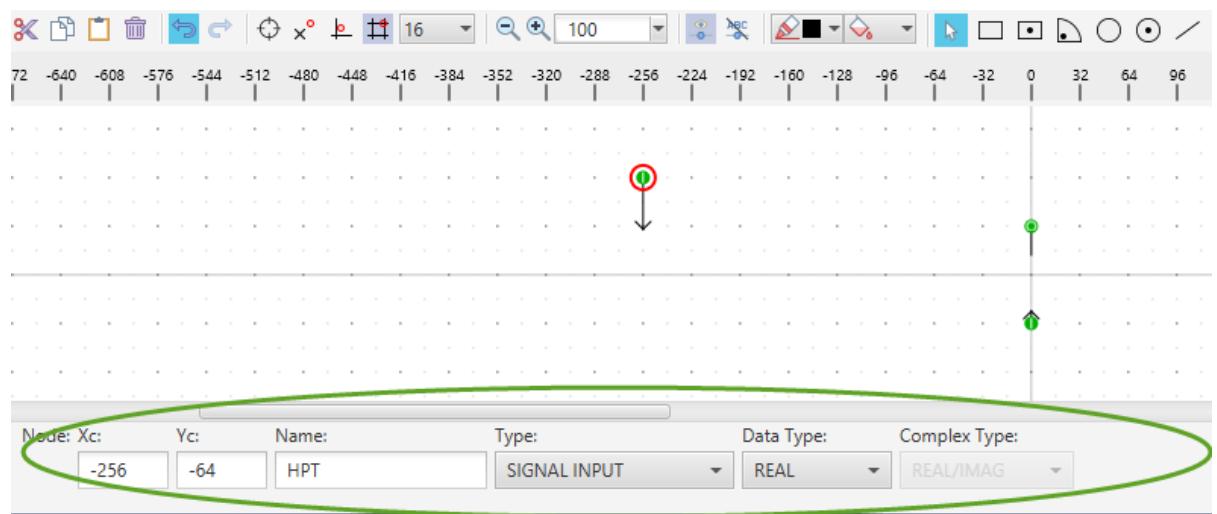
| b. Define the Input/Output points and associated conditional logic under the IO Points Tab | |
| Torque input for the HP Turbine, electrical Torque input to the generator and generator delta- omega output are always present. No logic needs to be placed around these input / output points. Select the create input/output point button from the drawing toolbar and left click when the circle is positioned as shown in Figure 4.9. Use the create input/output function to create points for the HPT input, The input and delta- omega output signals. A menu for the input/output point name and type (input or output, int or real) appears at the bottom when a input/output point is selected. All of the torque inputs are specified as real type. | |
|  | |
| Figure 4.9: IO Points | |
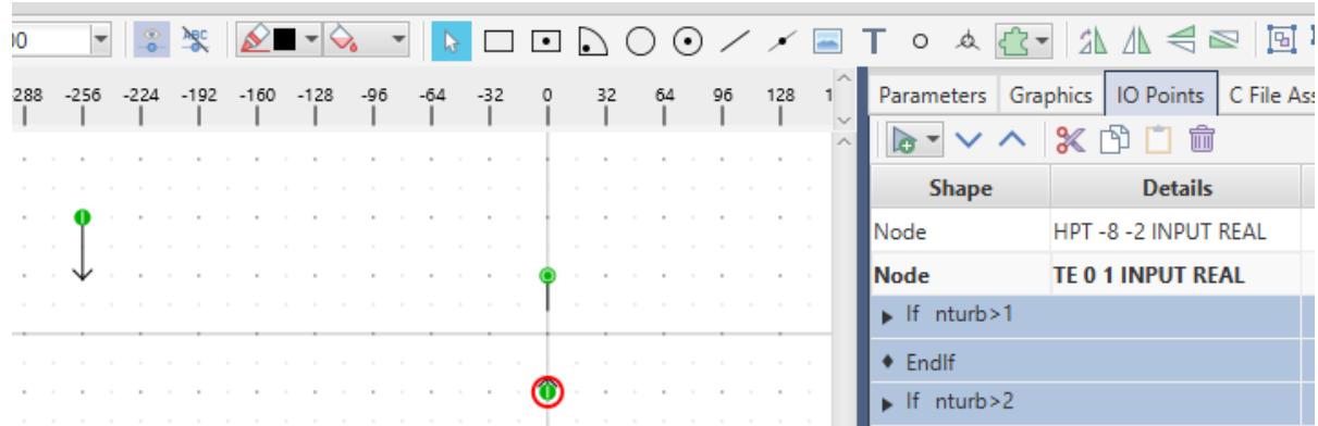
| The number of turbines included in each instance of the component is set by the user. Torque inputs for turbines other than for the HP turbine need to be placed inside conditional logic so that the inputs are enabled only when dictated by the number of selected turbines. To define a new condition, under the IO Points section, left click the add condition button and select the if option from the pull down. Enter the logic condition as shown below. The parameter nturnb, defined later, holds the number of turbines selected by the user. | |
|  | |
| Figure 4.10: Input/Output Points Details | |
| While the If (nturb>1) - EndIf block is highlighted in the IO Points section, add the input point for the IPA torque signal. The new input point is created inside the highlighted If- EndIf logic. | |
| Data under the IO Points tab should appear as shown in Figure 4.11 once all of the input / output points and associated logic has been entered. | |
| 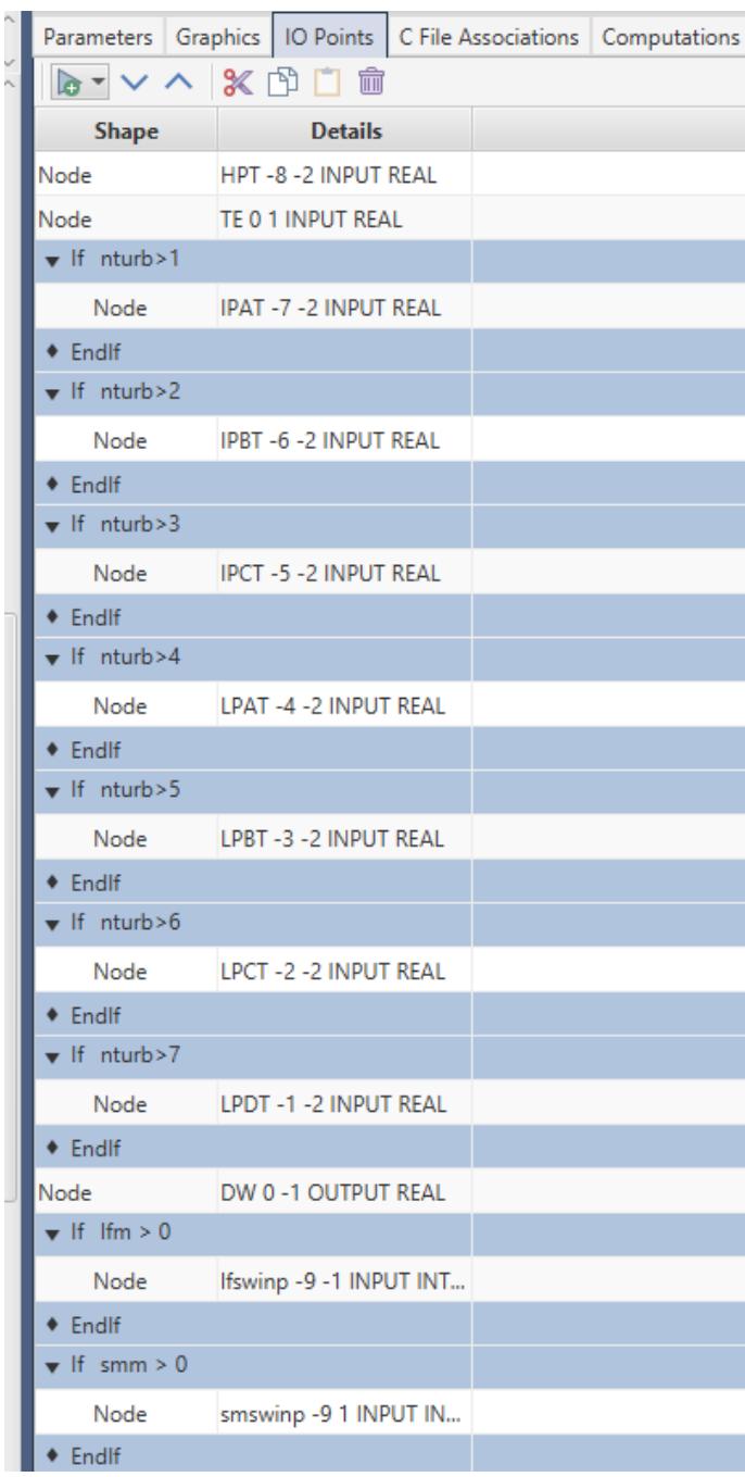 | |
| Figure 4.11:Data Under the I/O Points Tab | |
| c. Draw the unconditional graphics. | |
| d. Draw the conditional graphics. | |
| Turbine blocks which are not enabled are replaced by a shaft section for the component's appearance in RSCAD/Draft. Exciter masses are only drawn if enabled. L/F (Lock/Free) and S/M (Single/Multi) input wires are only drawn if the user selects these inputs are to come from a signal input rather than an RSCAD/RunTime switch. | |
| To add a logic condition under the Graphics tab select the Add Condition button and choose the if option from the pulldown. Enter the condition appropriate for the turbine section which is to be drawn within the logic condition. Since either a shaft section or turbine icon will be drawn, an if- else- endifstructure is required. To add an else section, highlight the newly created if- EndIf condition by left clicking on the If statement (the If and EndIf lines will turn red). Left click the Add Condition button and this time select Else from the pull down that appears. | |
| The condition logic should appear as follows - | |
| if (nturb>1) Else EndIf | |
| To add drawing commands into a particular condition, left click the small arrow next to the logic condition in which the drawing commands are to be placed. The condition turns red and the arrow should point downwards. Use the drawing commands to draw the shapes required for the icon portion. Drawing commands are placed within the highlighted logic condition. To draw the icon portion in the else section left click the small arrow next to the if line so that it again points to the right. The components drawn within the if section disappear from the drawing canvas. Now left click the small arrow next to the else line. The line becomes red and the arrow points downward. Draw the shapes required for the else portion of the icon. Repeat the above procedure for each turbine section. | |
| The multimass model permits representation of up to 2 rotating exciters. No torque input is applied to these exciter masses. A variable named "EXCen" is set to 0/1/2 by the user to indicate the number of exciter masses to be modelled. The logic for drawing the exciters can be arranged as follows - | |
| If (EXCen > 0) Draw shapes to represent exciter net to generator EndIf | |
| If (EXCen == 2) Draw shapes to represent 2nd exciter EndIf | |
| # 4.7.9 ADD PARAMETER ENTRY MENUS | |
| a. Now that the component icon, including input / output points and conditional graphics have been completed the menus for data entry are created. These menus are defined under the Parameters tab in the control pane area of the RSCAD/C-Builder window. | |
| The following sections are required for the multimass component. | |
| CONFIGURATION: basic configuration parameters including the number of turbines to be represented (nturb) and how many exciter masses are to be modelled (EXCen) SELF DAMPING: the self damping factors for each modelled mass. MUTUAL DAMPING: the damping factors for the shafts connecting the modelled masses. SHAFT SPRING CONSTANTS: the spring constants for the shafts connecting the modelled masses. INERTIA CONSTANTS: the inertia constants for each modelled mass. MASS SPEED MONITORING ENABLE: enable speed monitoring for each modelled mass. MASS SPEED SIGNAL NAMES: signal name for each monitored mass speed signal. MASS ANGLE MONITORING ENABLE: enable monitoring for the angle between each modelled mass. MASS ANGLE SIGNAL NAMES: signal name for each monitored mass angle signal. SHAFT TORQUE MONITORING ENABLE: enable shaft torque monitoring for each modelled shaft segment. SHAFT TORQUE SIGNAL NAMES: signal name for each monitored shaft torque signal. | |
| To create the component data entry sections listed above, left click the add section button in the control pane area of the RSCAD/C- Builder window. Enter the Section name in the menu that appears. | |
| None of the sections need an associated logic condition. | |
| Once all of the data entry sections have been created, left click the small arrow next to the section to which the parameters are to be added. The arrow points down and the section heading is highlighted. Left click the add parameter button and fill in the appropriate data in the menu that appears. The new parameter entry element is added under the highlighted section. | |
| 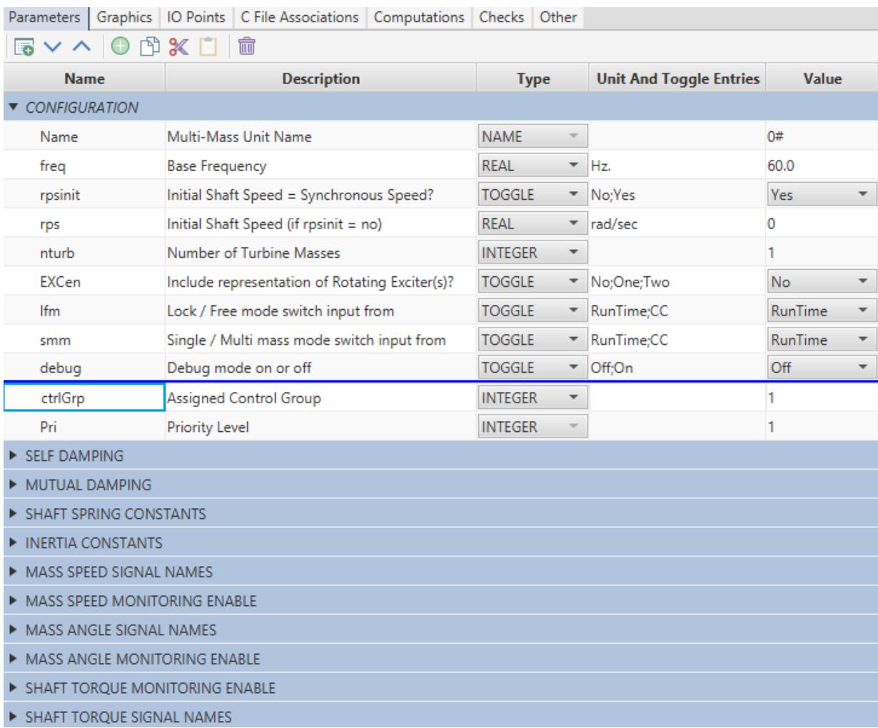 | |
| Figure 4.12: Parameters Tab | |
| b. Some parameters should only permit data entry when required. | |
| For example, if the user specifies that only 1 turbine mass is to be modelled (nturb = 1) then data for the IPA, IPB ... LPA turbine masses is not necessary and the associated parameters should not permit data entry. To facilitate this, a logic condition may be added to each parameter. | |
| To enable data entry for the IPA inertia constant only when the IPA turbine is to be modelled, add the following logic condition to the IPAH parameter entry - | |
| nturb>1 | |
| If the nturb parameter defined under the CONFIGURATION menu is set to 1 by the user then the IPAH parameter entry line will be greyed out. | |
| Names for monitored signals should only be entered if the associated turbine is modelled AND if the user has enabled that signal for monitoring. In this case the AND function can be used in the logic condition - | |
| nturb>1 &&HPIPATen | |
| # 4.7.10 WRITE DATA PREPARATION PORTION OF THE 'C' PROGRAM | |
| a. Create C File and Declare Variables | |
| There are two 'C' code programs that must be written by the user to complete the model. Firstly, a 'C' program which computes the constants required by the algorithm must be written. Secondly, the program which executes the algorithm for the model must be written. Only the second program runs on the RTDS hardware. Both 'C' programs are stored in the same file. A template for the 'C' file is created by selecting the "Add Model" button under the C File Associations tab. The newly created file can be edited by selecting the edit button. | |
| All of the input / output signals and parameters, as well as, their types are listed in a .h file which is automatically generated by C- Builder. The .h file is included as part of the 'C' code using the #include statement at the top of the 'C' code file. As such, all of the input / output and parameter signals may be used as part of the 'C' code. The simulation time- step may be obtained by adding the following statement into the 'C' code - | |
| The algorithm to be solved for the multimass model is essentially defined in equation 21 above. In order to solve [21] the following matrices must be computed as part of the data preparation code. | |
| <table><tr><td>[H], [D], [K]</td><td></td></tr><tr><td>[A], [B]</td><td></td></tr><tr><td>[A] -1</td><td></td></tr></table> | |
| The matrices are declared as double precision and dimensioned to the maximum number of masses (= 8 turbine masses + 1 generator mass + 2 exciter masses = 11 masses). | |
| RAM: #define MAXMASS 11 double H[MAXMASS][MASSMASS]; double K[MAXMASS][MASSMASS]; double D[MAXMASS][MASSMASS]; double A[MAXMASS][MASSMASS]; | |
| double B[MAXMASS][MASSMASS]; | |
| The above matrices are declared under the RAM: section in the 'C' code file since they are only used for the data preparation. The matrix Ainverse is required in both the data preparation and algorithm portions of the 'C' code and as such is declared under the STATIC: section of the 'C' code file. | |
| STATIC: double AINV[MAXMASS][MAXMASS]; | |
| # b. Load Data into Variables | |
| Data storage into the matrices and arrays is such that the lowest indexed entry is allocated to the High Pressure turbine. The next entry to the IP turbine and so on. Generator data is entered into the element pointed to by nturb. Exciter #1 is entered into the element pointed to by nturb+1. For example if the user has specified that four turbine masses are to be modelled (nturb=4) then the following code would be used to load the H matrix elements. Note that the inertia constants are loaded into the diagonal elements only and that off- diagonal elements of the H matrix are 0.0. | |
| $\begin{array}{rl}\mathbb{H}[0][0] & = \mathbb{HPH};\\ \mathbb{H}[1][1] & = \mathbb{IPAH}; \end{array}$ $\begin{array}{rl}\mathbb{H}[7][7] & = \mathbb{LPAH}; \end{array}$ H[ntrub][ntrub] $=$ GENH; H[ntrub+1][ntrub+1] $=$ EXC1H; H[ntrub+2][ntrub+2] $=$ EXC2H; | |
| The $D$ and $K$ matrices are tri- diagonal (see equation [22]) meaning that only their diagonal and diagonal $+ / - 1$ elements have non- zero values. Elements of these matrices are loaded one value at a time - | |
| D[0][0] $=$ HPSD $^+$ HPIPAMD; D[0][1] $=$ - HPIPAMD; D[1][0] $=$ - HPIPAMD; D[1][1] $=$ HPIPAMD $^+$ IPASD $^+$ IPAIPBMD; D[1][2] $=$ - IPAIPBMD; | |
| D[7][7] $=$ LPCLPDMD $^+$ LPDSD $^+$ LPGENMD; D[nturb][nturb] $=$ GENSD $^+$ LPGENMD; | |
| Exciter damping factors are added into nturb $^{+1}$ and nturb $^{+2}$ elements. | |
| Elements of the $K$ matrix are filled in using the same procedure as for the $D$ matrix. Once the $K,D$ and $H$ matrix elements are filled, the $A$ and $B$ matrices are computed as follows (see equation [19]). Computations are done only for the number of masses which are being modelled. | |
| nmass $=$ nturb $^{+1 + }$ EXCen; $\mathtt{K1} = \mathtt{4} / \mathtt{dt}$ $\mathtt{K2} = \mathtt{dt} / 2$ for (row $= 0$ ;row<nmass,row++) { for (col $= 0$ ;col<nmass;col++) { A[row][col] $= \mathbb{H}$ [row][col]\*k1+D[row][col] $^+$ K[row][col]\*k2; B[row][col] $= \mathbb{H}$ [row][col]\*k1- D[row][col] $^+$ K[row][col]\*k2; } } | |
| The inverse of the A matrix is required for the algorithm (see equation [21]). An internal matrix inversion routine is available to generate the required inverse matrix - | |
| $\dot{\texttt{i}} =$ matx invert(nmass,A,MAXMASS,AINV,MAXMASS); where - nmass $=$ dimension of matrix to invert $\mathtt{A} =$ matrix to invert MAXMASS $=$ dimension of matrices A and AINV $\mathtt{AINV} =$ matrix to store inverse of A | |
| The Ainv matrix is a full matrix. In addition to the Ainv matrix, the algorithm portion of the $^{\prime}C^{\prime}$ code also requires the B matrix and 2 times the k matrix. However, the B and $2^{n}k$ matrices are tri- diagonal and to conserve computations they will be stored in eleven separate arrays of dimension three. Each array holds the $n - 1$ n and $n + 1$ elements (where n is the diagonal element). Since these vectors are used in both the data preparation and algorithm portion of the $^{\prime}C^{\prime}$ code they are declared under the STATIC: section - | |
| STATIC: double K2TRIO[3], BTRIO[3]; double K2TRI1[3], BTRI1[3]; double K2TRI10[3], BTRI10[3]; | |
| The K2TRI and BTRI vectors are loaded from the K and B vectors. | |
| for $(\dot{1} = 0;\dot{1} < 3;\dot{1} + + )$ { BRTRIO[i] $=$ B[0][i]; K2TRI0= 2.0 \* K[0][i]; BTRI10[i] $=$ B[10][i+8]; K2TRI10[i] $=$ 2.0 \* K[10][i+8]; } | |
| c.Write Critical Data to the .map File | |
| It may be useful to include an option in the component's CONFIGURATION menu to print computed data into the .map file. Such data may be useful for debugging purposes during the model's development and testing, as well as, solving problems that may arise if third parties begin to use the model. | |
| Printing to the .map file may be done using the following structure of the fprintf statement | |
| fprintf(mapFile,"\n D[%d][%d] = %lf", row, col, D[row][col]); | |
| # 4.7.11 WRITE 'C' CODE TO IMPLEMENT THE ALGORITHM | |
| Now that all of the constants required for the algorithm have been computed, the 'C' code to implement the algorithm itself can be written. Code to execute the model algorithm is placed under the CODE: section in the 'C' file template. The basic structure of the code is as follows - | |
| variable declarations initializing If (mode $= =$ lock) { set all mass speeds } Else if (mode $=$ single) { solve one mass model } Else | |
| { compute multimass algorithm } write output signals | |
| The algorithm used to solve the multimass model is based on equation [21] (repeated below) and proceeds in the following steps. | |
| $$ | |
| [\omega_{n}(\tau)] = [A^{-1}]*[[T_{n}(\tau)] + [T_{n}(\tau -\Delta \tau)] + [B][\omega_{n}(\tau -\Delta \tau)] - [2K][\theta_{n}(\tau -\Delta \tau)] | |
| $$ | |
| 1. Compute $[BW] = [B]*[\omega (t - dt)]$ . Since only the non-zero elements of $[B]$ are stored the calculation is done as follows - | |
| $$ | |
| \left[ \begin{array}{c}BW_0\\ BW_1\\ BW_2\\ BW_3 \end{array} \right] = \left[ \begin{array}{cccc}B_{00} & B_{01} & 0 & 0\\ B_{10} & B_{11} & B_{12} & 0\\ 0 & B_{21} & B_{22} & B_{23}\\ 0 & 0 & B_{32} & B_{33} \end{array} \right]\left[ \begin{array}{c}Wold_0\\ Wold_1\\ Wold_2\\ Wold_3 \end{array} \right] | |
| $$ | |
| BW[0] $=$ BTRIO[0] \* wold[0] $^+$ BTRIO[1] \* wold[1]; BW[1] $=$ BTRI1[0] \* wold[0] $^+$ BTRI1[1] \* wold[1] $^+$ BTRI1[2] \* wold[2]; BW[2] $=$ BTRI2[0] \* wold[1] $^+$ BTRI2[1] \* wold[2] $^+$ BTRI2[2] \* wold[3]; BW[3] $=$ BTRI3[0] \* wold[2] $^+$ BTRI3[1] \* wold[3] $^+$ BTRI3[2] \* wold[4]; | |
| 2. Compute $[K2TH] = [K2]*[THold(t - dt)]$ . Since only the non-zeroelements of [K2] are stored the calculation is done as follows - | |
| $$ | |
| \left[ \begin{array}{c}K2TH_0\\ K2TH_1\\ K2TH_2\\ K2TH_3 \end{array} \right] = \left[ \begin{array}{cccc}K2_{00} & K2_{01} & 0 & 0\\ K2_{10} & K2_{11} & K2_{12} & 0\\ 0 & K_{21} & K2_{22} & K2_{23}\\ 0 & 0 & K2_{32} & K2_{33} \end{array} \right]\left[ \begin{array}{c}THold_0\\ THold_1\\ THold_2\\ THold_3 \end{array} \right] | |
| $$ | |
| K2TH[0] $=$ K2TRIO[0] \* THold[0] $^+$ K2TRIO[1] \* THold[1]; K2TH[1] $=$ K2TRI1[0] \* THold[0] $^+$ K2TRI1[1] \* THold[1] $^+$ K2TRI1[2] \* THold[2]; K2TH[2] $=$ K2TRI2[0] \* THold[1] $^+$ K2TRI2[1] \* THold[2] $^+$ K2TRI2[2] \* THold[3]; K2TH[3] $=$ K2TRI3[0] \* THold[2] $^+$ K2TRI3[1] \* THold[3] $^+$ K2TRI3[2] \* THold[4]; | |
| 3. Compute $[Bcol] = [Told] + [BW] - [K2TH]$ . $[BW]$ and $[K2TH]$ were computed in steps 1 and 2 above. $[Told]$ are the shaft torques computed in the previous time-step. $[Told]$ , $[BW]$ and $[K2TH]$ are column vectors and can thus $[Bcol]$ may be computed | |
| using a for loop as shown below - | |
| for (ii=0;ii<nmass;ii++) { $\mathtt{BCOL}[\mathtt{ii}] = \mathtt{T}[\mathtt{ii}] + \mathtt{BW}[\mathtt{ii}] - \mathtt{K2TH}[\mathtt{ii}];$ } | |
| 4. Compute $[\mathtt{Bcol}] = [\mathtt{Bcol}] + [\mathtt{T}]$ . The [T] vector is the latest shaft torques which must first be read in from the external source. Only those input torques associated with masses that are actually modelled may be read in. Once read, the new shaft torques can be added to the [BCOL] vector computed in step 3a. | |
| T[0] $=$ HPT; if (nturb $= = 8$ { T[1] $=$ IPAT; T[2] $=$ IPBT; T[3] $=$ IPCT; T[4] $=$ LPAT; T[5] $=$ LPBT; T[6] $=$ LPCT; T[7] $=$ LPDT; } else if (nturb $= = 7$ { } else if (nturb $= = 2$ { T[1] $=$ IPAT; } for (ii $= 0$ ;ii<nmass;ii++) { $\mathtt{BCOL}[\mathtt{ii}] = \mathtt{BCOL}[\mathtt{ii}] + \mathtt{T}[\mathtt{ii}];$ } | |
| 5. Compute [w] = [Ainv]*[BCOL]. Matrix [Ainv] is stored as a full nxn matrix and as such for loops can be used to compute the new mass speed vector [W]. | |
| for (ii=0;ii<nmass;ii++) { w[ii] $= 0,0$ for (jj=0;jj<nmass;jj++) { w[ii] $=$ w[ii] $^+$ Ainv[ii][jj]\*BCOL[jj]; } | |
| } | |
| 6. With the new speeds of each modelled mass known from step 4, it is now possible to compute the angles of each mass. The computed mass angles are used in step 2 during the next time-step in the computation of speed. The vector THold is used to store the newly computed values of mass angles. | |
| dt2= 0.5\*de1t; for (ii=0;ii<nmass;ii++) { THold[ii] $=$ THold[ii] $^+$ dt2\*(wold[ii] $^+$ w[ii]); } | |
| The generator mass angle is chosen as the reference (0 deg). The computed generator mass angle is subtracted from each modelled mass, including the generator mass itself. | |
| for (ii=0;ii<nturb;ii++) { THold[ii] $=$ THold[ii] - THold[nturb]; } THold[nturb+1] $=$ THold[nturb+1]- THold[nturb]; THold[nturb+2] $=$ THold[nturb+2]- THold[nturb]; THold[nturb] $=$ 0.0; | |
| 7. Now that the multimass algorithm has been solved, monitored variables can be prepared. All of the computations done within the algorithm are based on per-unit quantities. Monitored variables need to be converted to the desired units prior to being written out. The following conversions are done - | |
| [w] speed pu \* 2\*PI\*Base_Freq - > speed in rad/sec [THold] shaft angle in pu \*360 \* 2\*PI\*Base_Freq - > shaft angle in degrees | |
| Shaft torques are computed using the angle across the shaft. For example, to compute the torque across the shaft connecting the HP and IPA masses - | |
| HPIPAT $=$ HPIPAK \* (THold[0]- THold[1]) where HPIPAK is the spring constant for the shaft | |
| 8. Some additional code needs to be added to the algorithm to handle the lock/free switch. The Ifm parameter under the CONFIGURATION menu permits the user to select whether the lock/ free switch is automatically created by the model or whether an external signal | |
| connected to an input point controls the lock/free operating mode of the multimass model. To handle both input options a variable lfmode is created and assigned input from the external signal or from the automatically created RSCAD/RunTime switch depending upon the selection of the lfm parameter. If the lfm parameter is equal to 0 then an RSCAD/RunTime switch is automatically created, otherwise the lock/free signal is read from an input point. | |
| if (lfm > 0) { lfmode = lfswinp; } else { lfmode = lfsw; } | |
| Both the lfswinp and lfsw variables are defined in the .h file that is created when the component is compiled. | |
| When the lock/free signal is set to free (lfmode=0), the algorithm as defined in steps 1- 6 above is executed. When in lock mode (lfmode = 1) all modelled mass speeds are fixed. | |
| k3= 1.0; if (rpsinit == 0) k3 = rps/omo; if (lfmode == 1) { for (ii=0;ii<nmass;ii++) { w[ii] = k3; } } | |
| The variable k3 is set to 1.0 (ie. 1.0 per- unit speed represents synchronous speed) if the rpsinit parameter is set to synchronous speed (rpsinit == 1 (Yes)) by the user. If the rpsinit parameter is set to non- synchronous speed (rpsinit == 0 (No)) then the specified initial speed is used to compute the initial per- unit speed of the machine and this value is used for all of the modelled mass speeds when operating in lock mode. | |
| When in lock mode or within the first time steps, the angles of each modelled mass can be computed based on the torque applied to each mass and the shaft spring constant. If there is only one turbine mass then the angle between the turbine and the generator may be computed as - | |
| THold[0] = Te / LPGENK; | |
| Where Te is the torque applied to the generator LPGENK is the shaft spring constant between the generator and turbine. | |
| If two turbine masses are modelled the initial mass angles are computed as - | |
| THold[1] $=$ Te / LPGENK; THold[2] $=$ THold[1] $^+$ (Te- IPAT)/HIPPAK; | |
| Initial angles for the exciters are set to 0.0 since no external torque is applied to the exciters. | |
| If the mode switches are set so that the lock/free is free and single/ multi is set to single, then all of the modelled masses are considered as one lumped mass. The torque applied to the lumped mass is equal to the sum of torques read in and the inertia constant of the equivalent mass is equal to the sum of all the modelled mass inertia constants. Self damping terms for all modelled masses are summed to give an equivalent self damping factor for the equivalent mass. Mass speed is computed as - | |
| where $\begin{array}{rl} & {\tt w[0] = \tt C2^{\star}\tt w[0] + \tt C1^{\star}(\tt Ttotal - \tt Te);}\\ & {\tt w[1] = \tt w[0];} \end{array}$ C1= dt/ (2\*totH); $\mathrm{C2} = \mathrm{1.0} - \mathrm{(dt^{\star}totSD) / 2^{\star}totH)};$ | |
| # 4.7.12 TEST NEWLY DEVELOPED MODEL | |
| Testing of the multimass model can start by examining the output written to the .map file and see whether it matches hand calculations. Multiplication of the A matrix by its inverse to see whether the unity matrix is obtained checks whether the matrix inversion routine in the data preparation code was properly executed. | |
| Once the basic data preparation is verified, a number of simulation cases increasing in complexity may be run to verify the model's operation. It is useful to run the model in its simplest mode (single mass) and compare its dynamic response to that which is expected. | |
| As a final test, the multimass model is tested against the First Benchmark Case as described in [2]: | |
| # 4.8 REFERENCES | |
| [1] R. Farmer, A. Schwalb, "Navajo Project Report on Subsynchronous Resonance Analysis and Solutions", IEEE Transactions on Power Apparatus and Systems, Vol. PAS- 96, No. 4, July 1977, pp.1226- 1232. | |
| [2] IEEE Subsynchronous Resonance Task Force "First Benchmark Model for Computer Simulation of Subsynchronous Resonance", IEEE Transactions on Power Apparatus and Systems, Vol. PAS- 96, No. 5, Sept/Oct 1977, pp.1565- 1572. | |
| [3] IEEE SSR Working Group "Second Benchmark Model for Simulation of Subsynchronous Resonance", IEEE Transactions on Power Apparatus and Systems, Vol. PAS- 104, No. 5, May 1985, pp.1057- 1066. | |
| [4] P. Kundar, Power System Stability and Control, McGraw- Hill, 1994. | |
| [5] G. Gross and M.C. Hall, "Synchronous Machine and Torsional Dynamics Simulation in the Computation of Electromagnetic Transients", IEEE Transactions on Power Apparatus and Systems, Vol. PAS- 97, No. 4, July/Aug. 1978, pp.1074- 1086. (in particular Appendix & Discussion) | |
| # 5 MULTI-THREAD COMPONENT | |
| # 5.1 INTRODUCTION | |
| In real time digital power system simulation, the minimum length of time step used in the simulation is dictated by the most time- consuming algorithm which has to be completed in the time step. Provided the resulting time step is compatible with the bandwidth of the phenomena being investigated the simulation can run in real time. When a smaller time step is necessary to meet the bandwidth requirements the simulation can still run but not in real time. | |
| If the relay algorithm can be broken down into a number of independent blocks of code which can be evaluated sequentially in successive time steps and subsequently organized into a complete relay algorithm solution when all blocks have been evaluated then the time step used in the main simulation can be smaller than the time needed to run the complete relay algorithm. These blocks of code running in different time steps are called" threads" which are subsequently "woven" together to form the complete relay solution. Any component algorithm can be separated into individual blocks of code processed independently of each other to create a multi- threaded component running in the main simulation. The multi- threaded component requires additional code to keep track of the multi- threaded loop and adjust delays for timers when new sampled data is available. This additional code will ensure the individual blocks of code are executed sequentially, and restart the sequence when new sampled data is ready. | |
| This document outlines how the multi- threaded component can be incorporated into a model for use on the RTDS. Once the template for the multi- thread component is developed, the procedure for implementing some simple algorithms using the CBuilder feature under RSCAD is documented. | |
| # 5.2 MULTI-FUNCTION RELAYS | |
| 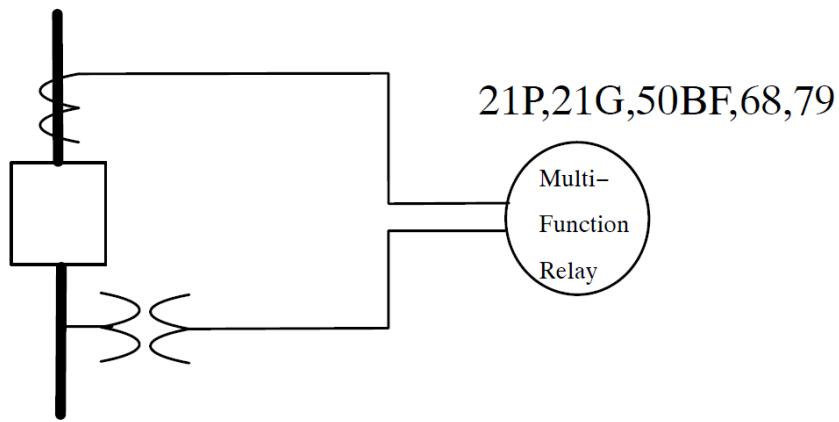 | |
| Figure 5.1: Multi-Functional Relay | |
| Normally a micro- processor based intelligent electronic device (IED) will use data sampled every 8/16/32/ or 64 samples per cycle. Relaying components are created using basic protection theory and standard techniques for processing digitally sampled data from the time domain. Essentially sampled data is transferred into the phase domain using a DFT or equivalent technique. The phasor information is then evaluated against algorithms that can discern between normal operating conditions and fault conditions. Control algorithms can then be processed that will isolate the faulted portion of the power system. The same control algorithm can then later restore the isolated portion of the power system when the fault condition has been removed. | |
| # 5.3 MULTI-THREAD COMPONENT | |
| A down- sampler is used to provide data at the correct number of samples per cycle for the algorithm. In an example case with a nominal $60\text{Hz}$ base sampling rate of 8 samples per cycle, the control algorithm obtains and uses new data every 2.08333 ms. If the simulation time- step is $50\mu \mathrm{sec}$ , then the main simulation will be executed 41 times between samples. This means that it is possible to have 41 different threads executed sequentially every 2.08333 ms. The execution time for a multifunctional relay algorithm without using threads will require the use of a longer simulation time step. If there are 5 threads in the multi- thread cycle with an additional thread every new sample the normal delay cycle between individual threads is $250\mu \mathrm{sec}$ . The additional thread every sample is normally used for the signal processing. This means the multi- thread cycle would execute about 7 times between new samples. Keep in mind that some code will be executed each time step and must be taken into consideration for overall execution time of each thread. The sample rate is not always an integer value of the time- step therefore new samples will occur with an | |
| accuracy limited to a few time- steps. This means that the thread cycle will restart at different thread counts changing the amount of delay between the executions of code within a thread. This delay can be adjusted from the normal 250 $\mu$ sec to a temporary value whenever the new data sample interrupts the thread cycle and restarts. | |
| 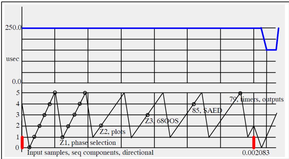 | |
| Figure 5.2: Multi-Threaded Time-Step | |
| If a timer is used in thread 1 the time between executions of thread 1 changes when a new sample occurs indicated by the red line. When the control algorithm is ready to read the new sample data, the multi- thread was executing thread 2. Because new sample data is ready to be read the control algorithm has to move back to thread 0 and read in and process the new sampled data that will be used for the other threads. | |
| When the multi- thread moves back to thread 1 and starts executing the code, only 3 main simulation timesteps have occurred. To properly service a timer in thread 1 the amount of delay added to the timer would have to be temporarily adjusted by 3/5 of the 250 $\mu$ sec (5 time- steps) normally added. | |
| The multi- thread component example will contain the necessary code to temporarily change the amount of time added to timers when a new sample occurs. | |
| # 5.4 MODEL DEVELOPMENT USING CBNIDLER | |
| Development of the multi- thread model requires the following steps: | |
| 1. Conceptual layout of the new component a) Which inputs should be connected using wires? b) Which outputs should be connected using wires? | |
| c) Appearance of the component icon. | |
| d) Options which change appearance of icon. | |
| e) What data is required to prepare the constants? | |
| f) How to group related data fields. | |
| g) What monitoring options should be available? | |
| 2. Component Icon Creation in C-Builder (Graphics & Nodes) | |
| a) Define component as a Control system type component. | |
| b) Locate and place all of the input/output points. | |
| c) Draw component icon. | |
| 3. Define User Supplied Data Menus (Parameters) | |
| a) Add all of the data sections defined under I(f) above. | |
| b) Add logic to parameters so the parameter entry fields are visible only when the corresponding options are selected. | |
| 4. Write Data Preparation Portion of the 'C' Program | |
| a) Create C File and Declare required variables. | |
| b) Compute constants required for the executable code. | |
| c) Optionally write critical data to the .map file. | |
| 5. Write 'C' code to implement the algorithm | |
| a) Declare required variables. | |
| b) Create variables for named output signals. | |
| c) Create variables for named input signals. | |
| 6. Test newly developed Model | |
| a) Check data preparation to ensure constants are computed correctly. | |
| b) Run simulation cases to confirm basic operation. | |
| 1. Conceptual Layout of the New Component | |
| a) Typically, controls components are drawn such that input points are on the left side and output points are on the right side of the component. | |
| b) The example model requires the name of an external variable to choose which thread's fractional delay is on output 7 (Frac). | |
| c) The component's appearance is shown below. IN1 - IN6 start the timers when 0 - >1 transition occurs on the inputs. | |
| IN1 - IN6 starts the timers | |
| Improve delay adjusts of the thread delay Frac Elapsed changes the outputs from elapsed time to the fraction delay for each thread Analog IP is the input for the sampler and DFT Timer- 1 to Timer- 6 is the output for each thread Frac is the output of the monitored thread Thread Count is the thread cycle Info is a word variable with the status of each timer | |
| 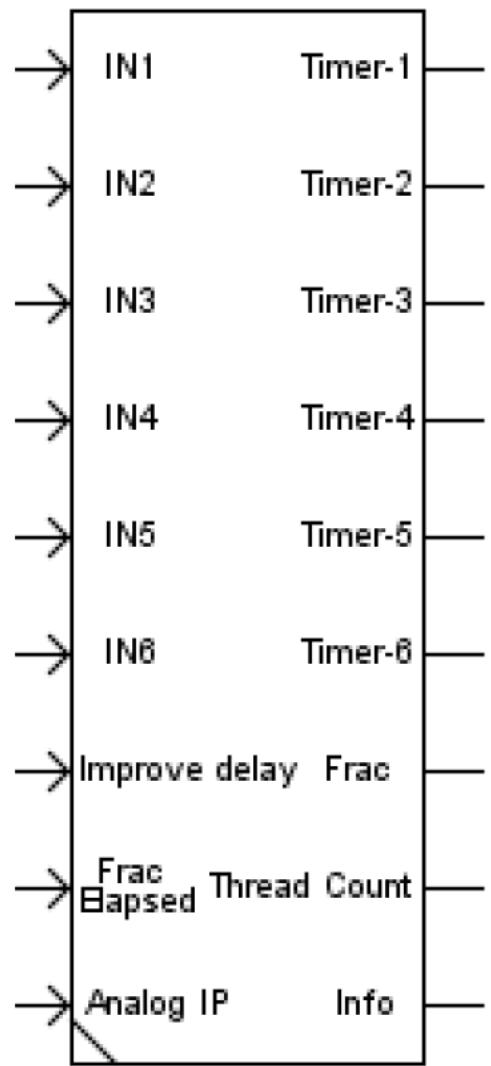 | |
| Figure 5.3: Multi Thread Component | |
| d) The following data tabs are defined for the multi-thread component: | |
| CONFIGURATION: Basic configuration options | |
| TIMERS: Time delay values for each timer | |
| MONITORING OPTION TAB: see below | |
| e) The user is able to select the following items for monitoring. These are named variables and as such there is no wire protruding from the component icon for any of these outputs. | |
| Trigger count when new sample occurs | |
| Analog input data | |
| Tabs are included in the component icon to facilitate selection of the signals to be monitored and the name assigned to each monitored variable. Logic is included | |
| as part of the component to permit selection of only those variables which are computed for the specified configuration. | |
| f) C-Builder requires that the user specify whether the component is a power system or control system type component. Power system components connect to power system nodes as defined by node icons in RSCAD/Draft and often contribute current injections into those nodes to which the component is connected. Control system components do not connect to power system nodes and are not able to supply current injections into the power system network. | |
| The Nova Cor to which a control system component is allocated automatically becomes a control system processor for the simulation case and only other control system components may be allocated to that processor. It is not possible to allocate both control system and power system components to the same NovaCor. | |
| # 2. Component Icon Creation in C-Builder | |
| The C- Builder User's Manual should be consulted for additional details on defining the component icon. Information provided here outlines the major steps required to complete the icon associated with the multi- thread model. | |
| a) Define the Component as a Control System Component. | |
| When a new component is created the user is prompted to select whether the component type is control or power system. For the multi- thread model select control. | |
| The component type can be changed anytime from the "Other" menu. | |
| Define the Input/Output points and associated conditional statements under the IO Points Tab. | |
| Inputs to start the timers are always present and require no conditional statements to be placed around these input/output points. Select the "Draw Node" button from the drawing toolbar and create points for the 6 inputs. All of the timer inputs are specified as integer type. | |
| 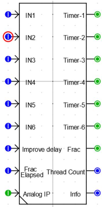 | |
| Figure 5.4: Component Icon in CBuilder | |
| Data under the IO Points tab should appear as shown in Figure 5.5 once all of the input/output points have been entered. The input/output points shown are outside logic conditions. | |
| 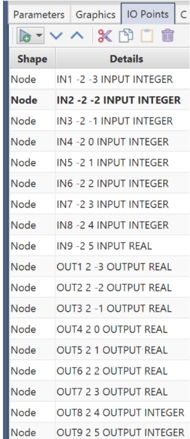 | |
| Figure 5.5: Data under IO Points Tab | |
| b) Draw the portions of the component icon which are outside of conditional logic. | |
| 3. Add Parameter Entries | |
| a) Now that the component icon, including input/output points and conditional graphics, has been completed the menus for data entry are created. These menus are defined under the Parameters tab in the control panel area of the RSCAD/C-Builder window. | |
| The following sections are required for the multi- thread component. | |
| CONFIGURATION: basic configuration parameters including the IED name, base frequency, variable name to choose value of OUT7, enable monitoring. | |
| TIMERS: pickup and dropout delay values for each timer. | |
| MONITORING: signal name for trigger count and signal name for analog input sampled data. Names for monitored signals should only be entered if plotting is enabled. | |
| plots $= 1$ | |
| To create the component data entry sections listed above, use the new section Parameters button in the control panel area of the RSCAD/C- Builder window. Enter the Section name in the menu that appears. None of the sections need an associated logic condition. | |
| Once all of the data entry sections have been created, left click the small arrow next to the section to which the parameters are to be added. The arrow points down and the section heading is highlighted. Left click the add parameter button and fill in the appropriate data in the menu that appears. The new parameter entry element is added under the highlighted section. | |
| 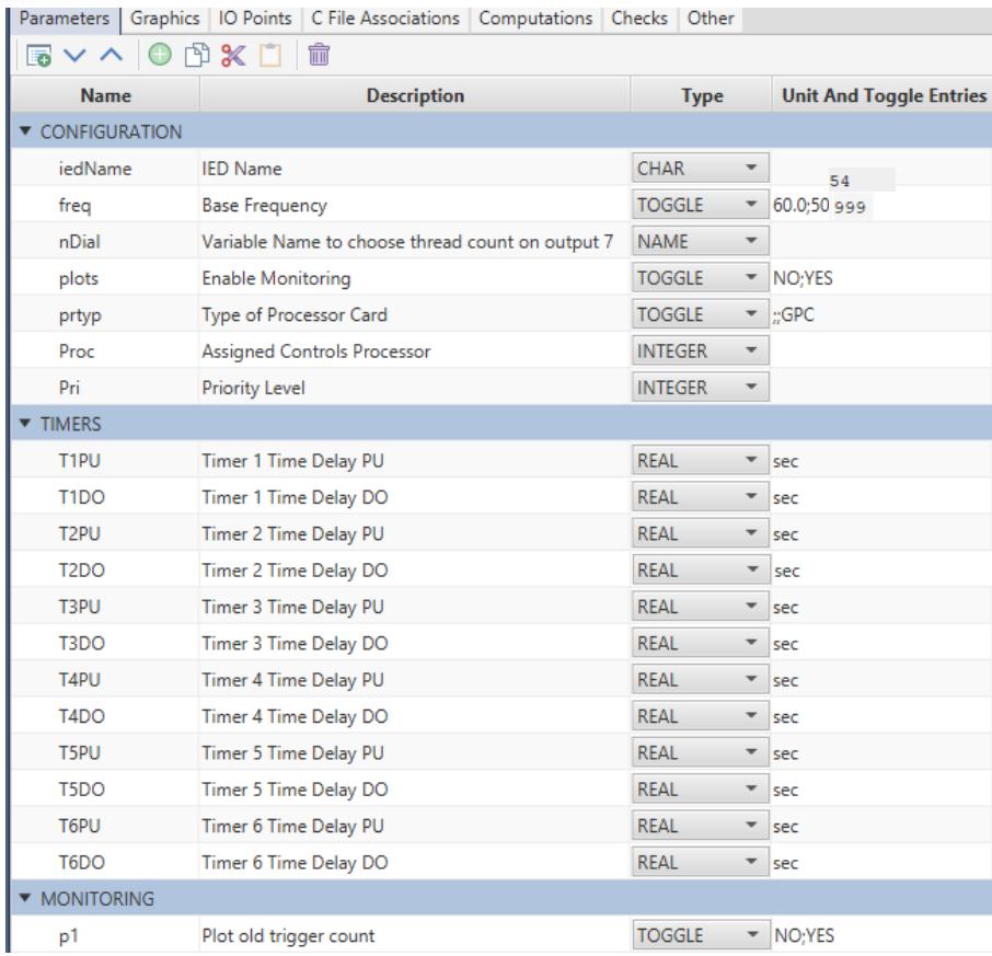 | |
| Figure 5.6: Adding Parameters | |
| # 4. Determine Ram Loader Code | |
| a) Some variables must change value when the base frequency changes. In this case the sample rate will change and the cutoff frequency will change when the base frequency changes. To facilitate this, a logic condition is added for each of the frequency parameter's state. | |
| To enable parameter changes relative to base frequency, add the following logic | |
| condition to the computations section. | |
| If the freq parameter defined under the CONFIGURATION menu is set to 1 (50 hz) by the user, then the SF parameter will be 0.400 and the fc variable will be 133.33. If the freq parameter is set to 0 (60 hz) then the SF parameter will be 0.480 and the fc variable will be 160.0. | |
| The parameter "freq" is added to the parameters section and used within the C program to change the 2 variables SF and fc. | |
| 5. Write Data Preparation Portion of the 'C' Programa) Create C File and Declare Variables. | |
| There are two $^{\prime}C^{\prime}$ code programs that must be written by the user to complete the model. First, a $^{\prime}C^{\prime}$ program which computes the constants required by the algorithm must be written. Secondly, the program which executes the algorithm for the model must be written. Only the second program runs on the RTDS hardware. Both $^{\prime}C^{\prime}$ programs are stored in the same file. A template for the $^{\prime}C^{\prime}$ file is created by selecting the "Add Model" button under the C File Associations tab. The newly created file can be edited by selecting the edit button. | |
| All of the input / output signals and parameters, as well as, their types are listed in a .h file which is automatically generated by C- Builder. The .h file is included as part of the $^{\prime}C^{\prime}$ code using the #include statement at the top of the $^{\prime}C^{\prime}$ code file. As such, all of the input / output and parameter signals may be used as part of the $^{\prime}C^{\prime}$ code. The simulation time- step may be obtained by adding the following statement into the $^{\prime}C^{\prime}$ code: | |
| $$ | |
| \mathsf{dt} = \mathsf{getTimeStep}(\mathsf{\Omega}); | |
| $$ | |
| The algorithm to be solved for the model is essentially a down sampler, a DFT, and timers. In order to run the anti- alias filter the constants must be computed as part of the data preparation code. As well the down sampler should have a sample rate relative to the base frequency. The RAM section will be used to perform all of the off- line section of code. | |
| b) Load Data into Variables. | |
| b) Load Data into Variables.The main portion DFT will use an 8-point buffer to determine the DC, fundamental, and second harmonic content of the analog input. The starting point of the buffer can be initialized such that the phasor will be at angle zero. | |
| c) Write Critical Data to the .map File | |
| It may be useful to include an option in the component's CONFIGURATION menu to print computed data into the .map file. Such data may be useful for debugging purposes during the model's development and testing, as well as, solving problems that may arise if third parties begin to use the model. | |
| Printing to the .map file may be done using the following structure of the fprintf statement: | |
| fprintf(mapFile,"\n D[%d][%d] = %lf", row, col, D[row][col]); | |
| 6. Write $^{\prime}C^{\prime}$ Code to Implement the Algorithm. | |
| Now that all of the constants required for the algorithm have been computed, the $^{\prime}C^{\prime}$ code to implement the algorithm itself can be written. Code to execute the model algorithm is placed under the CODE: section in the $^{\prime}C^{\prime}$ file template. The basic structure of the code is shown on pages in latter sections. | |
| # 7.Test Newly Developed Model | |
| Testing of the multi- thread model can start by examining the output of the timers with input 7 enabled or disabled. | |
| Once the basic data preparation is verified, a number of simulation cases increasing in complexity may be run to verify the model's operation. It is useful to run the model with a pure sine wave at base frequency and evaluate the plots to what is expected. | |
| # 5.5 MULTI-THREADMODELALGORITHM | |
| The algorithm for the multi- thread model is based on the above idea. The model will contain seven threads with a timer in six of the threads. The timers are activated when a value greater than O is applied to the appropriate input. The model will also contain code for data sampling and a DFT function. | |
| The main purpose here is not to develop a complex relay but to introduce a template which can be used to create multi- functional relays. | |
| // Processing Threads are: // 0 - Anti- alias filter, downsampler, DFT // 1 - Timer 1, phasor rotation and plots | |
| // 2 - Timer 2// 3 - Timer 3// 4 - Timer 4// 5 - Timer 5// 6 - Timer 6 | |
| # 5.6 MULTI-THREAD STATIC SECTION | |
| // Include file below is generated by C- Builder// and contains the variables declared as - // PARAMETERS, INPUTS, OUTPUTS...#include "PN_MT_temp.h" | |
| // time delay countersdouble tdpu_ip1,tdpu_ip2,tdpu_ip3;double tdpu_ip4,tdpu_ip5,tdpu_ip6;double tddo_ip1,tddo_ip2,tddo_ip3;double tddo_ip4,tddo_ip5,tddo_ip6; | |
| // Other variablesdouble dt,del,fracdel,nThread,nThreadInv;int sample_new,trig,trigcnt,trigcnt_old,nThreadInt;int ip1,ip2,ip3,ip4,ip5,ip6,ip7,ip8,nfrac,dthalf;int start1,start2,start3,start4,start5,start6;double va_re,va_im,va2_re,va2_im;double temp_re, temp_im, os1_1,os1_2;double inv_dt,bfreq,favg;double e_timer,f_timer,w_tan1,w_tan2,f_F13;double f_sample_t,meas1,meas1old,hold1,tmp;double va_buff[8]; | |
| int n_1[3], n_2[3], int idx; double FUND_FACTOR, DC_FACTOR, _2ND_FACTOR; double A[5], B[5], C[5], a_bre, a_bim; | |
| /\* - End of S TATIC: Section - \*/ | |
| # OUTPUTS: | |
| int cnt_old $=$ createOutput(nP1, strcat2("Relays|",iedName),0,100,"NA",p1&&plots); double A1RE $=$ createOutput(nP2r, strcat2("Relays|",iedName),0,100,"x",p2&&plots); double A1IM $=$ createOutput(nP2i, strcat2("Relays|",iedName),0,100,"y",p2&&plots); doubleA1FUND $=$ createOutput(nP2fm, strcat2("Relays|",iedName),0,100,"NA",p2&&plots); doubleA12ND $=$ createOutput(nP22nd, strcat2("Relays|",iedName),0,100,"NA",p2&&plots); double A1DC $=$ createOutput(nP2dc, strcat2("Relays|",iedName),0,100,"NA",p2&&plots); | |
| # 5.7 MULTI-THREAD RAM SECTION | |
| int i,k,nsn; double nsf,wcp,cosn,x; | |
| if(freq $\scriptstyle \mathbf{\omega} = =0$ { $\mathsf{SF} = 0.480;$ $\mathsf{fc} = 160.0;$ }else{ $\mathsf{SF} = 0.400;$ $\mathsf{fc} = 133.33;$ } dt $=$ getTimeStep();// Simulation time step nThreadInt $= 7$ nThread $= 7.0$ nThreadInv $= 1.0$ /nThread; | |
| fracdel $=$ nThread \* dt;// RSCAD time step,delay is multiple # of threads del $=$ fracdel; dthalf $= 0.5^{*}$ det; // Pick Up Delay Calculation tdpu_ip1 $= 0.0$ tdpu_ip2 $= 0.0$ tdpu_ip3 $= 0.0$ tdpu_ip4 $= 0.0$ tdpu_ip5 $= 0.0$ tdpu_ip6 $= 0.0$ tddo_ip1 $= 0.0$ tddo_ip2 $= 0.0$ tddo_ip3 $= 0.0$ tddo_ip4 $= 0.0$ tddo_ip5 $= 0.0$ tddo_ip6 $= 0.0$ $\mathsf{ip1} = 0;$ $\mathsf{ip}2 = 0;$ $\mathsf{ip}3 = 0;$ $\mathsf{ip}4 = 0;$ $\mathsf{ip}5 = 0;$ $\mathsf{ip}6 = 0;$ $\mathsf{ip}7 = 0;$ $\mathsf{ip}8 = 0;$ start1 $= 0$ start2 $= 0$ start3 $= 0$ start4 $= 0$ start5 $= 0$ start6 $= 0$ | |
| // INPUT processing Initialization\n\n\n\n\n\n\n\n\n\n\n\n\n\n\n\n\n\n\n\n\n\n\n\n\n\n\n\n\n\n\n\n\n\n\n\n\n\n\n\n\n\n\n\n\n\n\n\n\n\n\n\n\n\n\n\n\n\n\n\n\n\n\n\n\n\n\n\n\n\n\n\n\n\n\n\n\n\n\n\n\n\n\n\n\n\n\n\n\n\n\n\n\n\n\n\n\n\n\n\n\)\mathsf{nsn}=1;\(\)\mathsf{nsf}=1.0;\(\)\mathsf{inv\_dt}=1.0/\mathsf{dt};\(\)\mathsf{f\_sample\_t}=0.001/\mathsf{SF};\(\)\mathsf{bfreq}=\mathsf{SF}^*125.0;\(\)\mathsf{favg}=\mathsf{bfreq};\(\)\mathsf{idx}=6;//6\(samples to rotate by 270, normalizes Aph to 0.0 deg\)\mathsf{e\_timer}=0.0;//\(timer to enable freq tracking\)\mathsf{f\_timer}=10.25^*\mathsf{dt};\(/adjustment to help zero the phase\)\mathsf{//LP Filter constants calculations for(\)\mathsf{k}=0;\(\)\mathsf{k}<\mathsf{nsn};\(\)\mathsf{++k}\)\)\{\(\)\mathsf{wcp}=\sin(\mathsf{fc}*\mathsf{PI}*\mathsf{dt})/\cos(\mathsf{fc}*\mathsf{PI}*\mathsf{dt});\(\)\mathsf{cosn}=\cos((2.0^*(\mathsf{k}+\mathsf{nsf}+1.0)- 1.0)^*\mathsf{PI}/(4.0^*\mathsf{nsf}));\(\)\mathsf{x}=1.0/(1.0+\mathsf{wcp}^*\mathsf{wcp}- 2.0^*\mathsf{wcp}^*\mathsf{cosn});\(\)\mathsf{A}[\mathsf{k}]=\mathsf{wcp}^*\mathsf{wcp}^*\mathsf{x};\(\)\mathsf{B}[\mathsf{k}]=2.0^*(\mathsf{wcp}^*\mathsf{wcp}- 1.0)^*\mathsf{x};\(\)\mathsf{C}[\mathsf{k}]=({1.0}+\mathsf{wcp}^*\mathsf{wcp}+2.0^*\mathsf{wcp}^*\mathsf{cosn})^*\mathsf{x};\)\(\)\}\(\)\mathsf{for}(\mathsf{i}=0;\mathsf{i}<8;\mathsf{i}++)\(\)\{\(\)\mathsf{va\_buff[i]=0.0};\(\)\}\(\)\mathsf{FUND\_FACTOR}=0.176776695;//\(\)\mathsf{for}\(\)\mathsf{RMS}=>0.5^*(1/\mathsf{sqrtN})\(\)\mathsf{FUND\_FACTOR}=\mathsf{FUND\_FACTOR}^*1.009910335;//\(\)\mathsf{adjust}\(for the loss in the BW Filt at 160.0\)\mathsf{FC}\(\)\mathsf{2ND\_FACTOR}=\mathsf{FUND\_FACTOR}^*1.135933359;//\(\)\mathsf{adjust}\(for the loss in the BW Filt\)\mathsf{DC\_FACTOR}=0.125;\(\)\mathsf{/*}\mathrm{- - - - End}\mathsf{of}\mathsf{RAM}\colon\mathsf{S}\(ection\)\mathrm{- - - - }^*/$ | |
| # 5.8 MULTI-THREADCODESECTION | |
| meas1 = IN9; // Butterworth Filter for anti- aliasing 2nd order LP // VA first stage tmp = - B[0] \* os1_1 + - C[0] \* os1_2 + A[0] \* meas1; meas1 = tmp + 2.0 \* os1_1 + os1_2; os1_2 = os1_1; os1_1 = tmp; meas1old $=$ hold1; f_F13 = f_timer; e_timer $=$ e_timer $^+$ dt; f_timer $=$ f_timer $^+$ dt; if(f_timer > f_sample_t) { // linear interpolation tmp $=$ ((meas1 - meas1old) \* inv_dt) \* (f_sample_t - f_F13); meas1 $=$ tmp $^+$ meas1old; //8 SAMPLE BUFFER va_buff[idx] $=$ meas1; idx $=$ idx+1; idx $=$ idx % 8; // DFT FOR THE VOLTAGES AND CURRENTS A1DC $\equiv$ (va_buff[0]+va_buff[1]+va_buff[2]+va_buff[3]+va_buff [4]+va_buff[5]+va_buff[6]+va_buff[7])\*DC_FACTOR, va_re=(va_buff[0]- va_buff[4]+ INV_ROOT2\*(va_buff[1]- va_buff[3]- va_buff[5]+va_buff[7])) \*FUND_FACTOR; va_im $=$ (- va_buff[2]+va_buff[6]+INV_ROOT2\*(- va_buff[1]- v a_buff[3]+va_buff[5]+va_buff[7]))\*FUND_FACTOR; va2_re $=$ (va_buff[0]- va_buff[2]+va_buff[4]- va_buff[6])\*_2ND_FACTOR; | |
| va2_im $=$ - va_buff[1]+va_buff[3]- va_buff[5]+va_buff[7] \* 2N D_FACTOR; | |
| trig $= 1$ f_timer $= f$ timer- f_sample_t; trigcnt_old $=$ trigcnt; trigcnt $= 0$ sample_new $= 1$ // set the values for Inputs ip1 $=$ IN1; ip2 = IN2; ip3 = IN3; ip4 = IN4; ip5 = IN5; ip6 = IN6; ip7 = IN7; ip8 = IN8; } else { trig $= 0$ hold1 $=$ meas1; trigcnt $=$ trigcnt $+1$ if (trigcnt $>$ nThreadInt){ sample_new $= 0$ . trigcnt $= 1$ ; // go to Thread 1 } // // // // // // // // // // // // // // // // // // // // // // // // // // // // // // // // // // // // // // // // // // // // // // // // // // // // // // // // // // // // // // // // // // // // // // // // // // // // // // // // // // // // // // // // // // // // // // // // // // // // if (trigcnt $= = 1$ { if (sample_new $= = 1$ ){ | |
| if (trigcnt_old<trigcnt){ fracdel $=$ (trigcnt $^+$ trigcnt_old $+5$ )\*nThreadInv\*del; } if (trigcnt_old $=$ =trigcnt){ fracdel $=$ (trigcnt_old $+1$ )\*nThreadInv\*del; } if (trigcnt_old $\gimel$ trigcnt){ fracdel $=$ (trigcnt_old $+1$ )\*nThreadInv\*del; } if (e_timer>0.1&& ip7>0){ w_tan1 $=$ atan2(va_im,va_re); // figure out the real and imag,then rotate the phasors a-bre $=$ cos(w_tan1); a_bim $=$ - sin(w_tan1); temp_re=(va_re \* a_bre)- (va_im \* a_bim); temp_im=(va_re \* a_bim) $^+$ (va_im \* a_bre); va_re $=$ temp_re; va_im $=$ temp_im; } } else { fracdel $=$ del; } // set the values for plots A1RE $=$ va_re; A1IM $=$ va_im; A1FUND $=$ sqrt((va_re \* va_re) $^+$ (va_im \* va_im)); | |
| A12ND $=$ sqrt((va2_re \* va2_re) $^+$ (va2_im \* va2_im)); } // // // // // // // // // // // // // // // // // // // // // // else if (trigcnt $= = 2$ { if (sample_new $= = 1$ && ip7>0){ if (trigcnt_old<trigcnt){ fracdel $=$ (trigcnt $^+$ trigcnt_old $+5$ )\*nThreadlnv\*del; } if (trigcnt_old $= =$ trigcnt){ fracdel $=$ (trigcnt_old $+1$ )\*nThreadlnv\*del; } if (trigcnt_old $>$ trigcnt){ fracdel $=$ (trigcnt_old $+1$ )\*nThreadlnv\*del; } } else { fracdel $=$ del; } // set the outputs for Timer 1 if $(\mathsf{ip}1 > 0)$ if (tdpu_ip1 $<$ T1PU){ tdpu_ip1 $=$ tdpu_ip1 $^+$ fracdel; } if (tdpu_ip1 $> =$ T1PU){ start1 $= 1$ } } | |
| else { if (start1 > 0){ tddo_ip1 = tddo_ip1 + fracdel; } if (tddo_ip1 >= T1DO){ start1 = 0; tdpu_ip1 = 0.0; tddo_ip1 = 0.0; } }// end of setoutputs if statement if (ip8 == 1){ OUT1 = fracdel; } else { if (ip1 > 0){ OUT1 = tdpu_ip1; } else { OUT1 = tddo_ip1; } } ///////////////// THREAD 3 ///////////////// ///////////////// else if (trigcnt == 3){ if (sample_new == 1 && ip7 > 0){ | |
| if (trigcnt_old<trigcnt){ fracdel $=$ (trigcnt $^+$ trigcnt_old $+4$ )\*nThreadInv\*del; } if (trigcnt_old $= =$ trigcnt){ fracdel $=$ (trigcnt_old $+1$ )\*nThreadInv\*del; } if (trigcnt_old>trigcnt){ fracdel $=$ (trigcnt_old $+1$ )\*nThreadInv\*del; } } else { fracdel $=$ del; } // CODE AS PER TIMER 1 } // // // // // // // // // // // // // // // // // // // // // // // // // // // // // // // // // // // // // // // // // // // // // // // // // // // // // // // // // // // // // // // // // // // // // // // // // // // // // // // // // // // // // // // // // // // // // // // // // // // // else if (trigcnt $= = 4$ { if (sample_new $= = 1$ && ip7>0){ if (trigcnt_old<trigcnt){ fracdel $=$ (trigcnt $^+$ trigcnt_old $+3$ )\*nThreadInv\*del; } if (trigcnt_old $= =$ trigcnt){ fracdel $=$ (trigcnt_old $+1$ )\*nThreadInv\*del; } if (trigcnt_old>trigcnt){ fracdel $=$ (trigcnt_old $+1$ )\*nThreadInv\*del; } } | |
| else { fracdel $=$ del; } // CODE AS PER TIMER 1 } //THREAD 5 //else if (trigcnt $= = 5$ { if (sample_new $= = 1$ && ip7>0){ if (trigcnt_old<trigcnt){ fracdel $=$ (trigcnt $^+$ trigcnt_old $+3$ )\*nThreadInv\*del; } if (trigcnt_old $= =$ trigcnt){ fracdel $=$ (trigcnt_old $+1$ )\*nThreadInv\*del; } if (trigcnt_old>trigcnt){ fracdel $=$ (trigcnt_old $+1$ )\*nThreadInv\*del; } } else { fracdel $=$ del; } // CODE AS PER TIMER 1 } //THREAD 6 //else if (trigcnt $= = 6$ { if (sample_new $= = 1$ && ip7>0){ if (trigcnt_old<trigcnt){ fracdel $=$ (trigcnt $^+$ trigcnt_old $+2$ )\*nThreadInv\*del; | |
| } if (trigcnt_old $=$ =trigcnt){ fracdel $=$ (trigcnt $+1$ )\*nThreadInv\*del; } } else { fracdel $=$ del; }//CODE AS PER TIMER 1 } ////////////////////////////////////////////////////////////////////////////////////////////////////////////////////////////////////////////////////////////////////////////////////////////////////////// ////////////////////////////////////////////////////////////////////////////////////////////////////////////////////////////////////////////////////////////////////////////////////////////////////// // /////////////////////////////////////////////////////////////////////////////////////////////////////////////////////////////////////////////////////////////////////////////////////////////////////// ////////////////////////////////////////////////////////////////////////////////////////////////////////////////////////////////////////////////////////////////////////////////////////////////////// /////////////////////////////////////////////////////////////////////////////////////////////////////////////////////////////////////////////////////////////////////////////////////////////////////// / ////////////////////////////////////////////////////////////////////////////////////////////////////////////////////////////////////////////////////////////////////////////////////////////////////// | |
| # 6 PMU SHELL COMPONENT | |
| # 6.1 INTRODUCTION | |
| In real time digital power system simulation, the minimum length of time step used in the simulation is dictated by the most time- consuming algorithm which has to be completed in the time step. Provided the resulting time step is compatible with the bandwidth of the phenomena being investigated the simulation can run in real time. When a smaller time step is necessary to meet the bandwidth requirements the simulation can still run but not in real time. | |
| This document describes the implementation of a Phasor Measurement Unit (PMU) algorithm using techniques introduced in tutorial chapter 5. | |
| This document outlines how the create the PMU shell from the source files found in the RSCAD installation directory. | |
| # 6.2 PHASOR MEASUREMENT UNIT | |
| 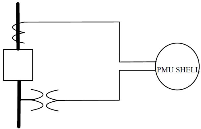 | |
| Figure 6.1:PMU AC Connection | |
| 6.2 PHASOR MEASUREMENT UNITPMUs are available from virtually every manufacturer of protection and monitoring equipment. They are often implemented as embedded functions within relays or disturbance recorders. This document describes a PMU shell software model for use on a Real Time Digital Simulator (RTDS). The algorithms that are part of the PMU shell are developed using the signal processing reference model from IEEE C37.118.1- 2011 Annex C. | |
| Development of a C- Builder model involves many steps and generally requires weeks or months from start to finish. The next page provides an overview of the steps typically involved to develop a model. | |
| RTDS has provided the source files that can be used by individuals to start developing their own PMU signal processing algorithms with C- builder and the GTNET- PMU firmware. | |
| # 6.3 MODEL DEVELOPMENT USING CBEULDER | |
| Development of the multi- thread model requires the following steps: | |
| 1. Conceptual layout of the new component | |
| a) Which inputs should be connected using wires? | |
| b) Which outputs should be connected using wires? | |
| c) Appearance of the component icon. | |
| d) Options which change appearance of icon. | |
| e) What data is required to prepare the constants? | |
| f) How to group related data fields. | |
| g) What monitoring options should be available? | |
| 2. Component Icon Creation in C-Builder (Graphics & Nodes) | |
| a) Define component as a Control system type component. | |
| b) Locate and place all of the input/output points. | |
| c) Draw component icon. | |
| 3. Define User Supplied Data Menus (Parameters) | |
| a) Add all of the data sections defined under I(f) above. | |
| b) Add logic to parameters so the parameter entry fields are visible only when the corresponding options are selected. | |
| 4. Write Data Preparation Portion of the 'C' Program | |
| a) Create C File and Declare required variables. | |
| b) Compute constants required for the executable code. | |
| c) Optionally write critical data to the .map file. | |
| 5. Write 'C' code to implement the algorithm | |
| a) Declare required variables. | |
| b) Create variables for named output signals. | |
| c) Create variables for named input signals. | |
| 6. Test newly developed Model | |
| a) Check data preparation to ensure constants are computed correctly. | |
| b) Run simulation cases to confirm basic operation. | |
| # 6.4 PMU SHELL COMPONENT | |
| C- Builder is used to create models that are not part of the normal RSCAD library. The source files are created and stored in the RSCAD user's root folder. | |
| The source files for the PMU SHELL component are installed in the installation directory of RSCAD. In this case it is assumed it is in C drive: C:\RSCAD_FX\EXAMPLES\TUTORIAL\CBuilder\CH- 6- PMU_SHELL\RTDS_USER | |
| There are 2 sub folders .\CMODEL_SOURCE and ..\ULIB, the "cmodel_source" folder contains the \*.c and \*.h files while the "ulib" folder contains the component definition file. | |
| The source files need to be copied to the RTDS, USER directory as follows: | |
| 1. Copy the file: C:\RSCAD_FX\EXAMPLES\TUTORIAL\CBuilder\CH-6-PMU_SHELL\RTDS_USER\ULIB\rt ds_GTNET_PMU_shell.def to your ULIB folder C:\RTDS_USER\ULIB\ | |
| 2. Copy the file: C:\RSCAD_FX\EXAMPLES\TUTORIAL\CBuilder\CH-6-PMU_SHELL\RTDS_USER\CMODEL _SOURCE\PMU_m.c to your BIN folder C:\RTDS_USER\BIN\CMODEL_SOURCE | |
| 3. Copy the file: C:\RSCAD_FX\EXAMPLES\TUTORIAL\CBuilder\CH-6-PMU_SHELL\RTDS_USER\CMODEL _SOURCE\PMU_m.h to your BIN folder C:\RTDS_USER\BIN\CMODEL_SOURCE | |
| 4. Copy the file: C:\RSCAD_FX\EXAMPLES\TUTORIAL\CBuilder\CH-6-PMU_SHELL\RTDS_USER\CMODEL _SOURCE\PMU_p.c to your BIN folder C:\RTDS_USER\BIN\CMODEL_SOURCE | |
| 5. Copy the file: C:\RSCAD_FX\EXAMPLES\TUTORIAL\CBuilder\CH-6-PMU_SHELL\RTDS_USER\CMODEL _SOURCE\PMU_p.h to your BIN folder C:\RTDS_USER\BIN\CMODEL_SOURCE | |
| # 6.5 LOAD PMU SHELL INTO CBuilder | |
| Start CBuilder and open the PMU shell component definition file: "_rtds_GTNET_PMU_shell.def". Once the component is loaded into CBuilder, the source files need to be compiled. | |
| Select the "C File Associations" tab (see 1 of Figure 6.2) and then click on the edit button for the PMU_p model (see 2 of Figure 6.2). Then click on the Compile button (see 3 of Figure 6.2). | |
| Repeat the following steps for PMU_M. | |
|  | |
| Figure 6.2: Compiling PMU Shell Source Files in CBuilder | |
| # 6.6 PMU SHELL ALGORITHM | |
| The PMU model developed to run on the RTDS includes the P class and M class reference models from the IEEE standard C37.118.1. Annex C. Figure 3 shows the typical steps used within the reference PMU to process the input signals [1]. A GTSYNC card provides the absolute time- reference and the simulation data is sampled using a fixed sample rate. The quadrature oscillator operates at nominal frequency and is used to perform complex multiplication of the input signal. The LP filters are Finite Impulse Response (FIR) and remove the double frequency component thus leaving the Re and Im part of the original input signal. For P and M class the LP filters are implemented using symmetrical FIR filters with an odd number of stages. The P class filter coefficients are calculated using a triangular window and the M class filter coefficients are calculated using windowed "sinc" function multiplied with a Hamming window. Each sample is time- stamped and compensated for the group delay of the LP filter. The phasor estimate at the center of the estimation window is unbiased by the actual system frequency and does not require further phase correction when the time- stamp at the center of the window is used. In IEEE C37.118.1- 2011 Annex C the P class samples data at 15 samples per cycle and the M class samples data at 16 samples per cycle at nominal frequency. We have modified the P class to sample at 16 samples per cycle so we can use higher reporting rates. | |
| 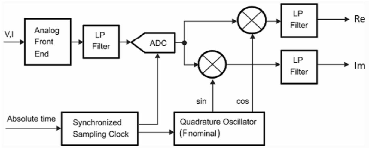 | |
| Figure 6.3: PMU Phasor Signal Processing Reference Model | |
| Although the block diagram in Figure 6.3 explains the concept of the reference model quite well, there are some subtle changes that need to be done for it to work on a real time digital simulator. The simulation data must be interpolated when sampled because the PMU sample rate may not be an integer multiple of the simulation time- step. The quadrature oscillator must also be interpolated by the same amount as the simulation data. The maximum reporting latency allowed by C37.118.1- 2011 is 2/Fs for P class and 5/Fs for M class where Fs is the reporting rate [2]. Therefore, the LP filter order must have latency less than the maximum allowed by the standard and also allow for other delays. The LP filter order can be quite large at the lower reporting rates and exceed the amount of available RAM. For example, an M class PMU operating at nominal 50Hz with a reporting rate of 10Fs requires a filter order of 700. The number of variables for just one PMU would be equal to 12,618. Because the RTDS model was designed to support 8 PMUs the amount of variables just to process the FIR filters would equal 100,944 for a 50HzMclass PMU reporting at 10Fs. During development of the RTDS PMU model the lowest supportable reporting rate was found to be 10Fs at 50Hz. As the reporting rates become lower the filter window length becomes larger to the point that the available memory limit is exceeded. The standard reference model does not provide filter parameters for reporting rates higher than 100Fs or 120Fs. In order to provide reporting rates at 200Fs and 240Fs for 50Hz and 60Hz respectively a 30 tap FIR filter using Dolph- Chebyshev coefficients was used. | |
| 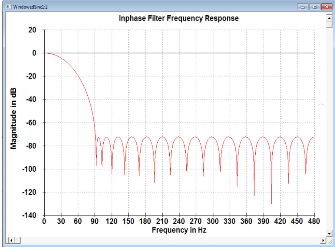 | |
| Figure 6.4: Magnitude Response of 240 frames/second Filter | |
| The processing of the simulation data and manipulation of the data into the format defined by the IEEE standard is computed on a NovaCor. Because each of the eight PMUs operating on the RTDS is independent, it is possible that all eight PMUs may output data at the same time. Therefore, a method to limit servicing of one PMU per simulation time- step was needed; to prevent buffer overflows on the GTNET. When PMU data is ready to be sent to the GTNET a service interrupt flag is set and is cleared once the PMU data is sent to the GTNET. | |
| # 6.7 C CODE SECTIONS | |
| The two *c files have been prepared to use the parameters specified in the PMU Shell component definition file. There are some very specific sections that SHOULD NOT BE MODIFIED! | |
| Before the | |
| //!!! DO NOT CHANGE THIS!!! | |
| STATIC: | |
| //GTNET PHASOR ARRAY variables //INPUT processing variables // FIR coefficients etc... | |
| The basic | |
| INPUTS: | |
| OUTPUTS: | |
| RAM_PASS1: | |
| RAM_PASS2: | |
| DOWNLOAD_FILE_CODE: | |
| //\*\*\*\*\*\*\*\*\*\*\*\*\*\*\*\*\*\*\*\*\*\*\*\*\*\*\*\*\*\*\*\*\*\*\*\*\*\*\*\*\*\*\*\*\*\*\*\*\*\*\*\*\*\*\*\*\*\*\*\*\*\*\*\*\*\*\*\*\*\*\*\*\*\*\*\*\*\*\*\*\*\*\*\*\*\*\*\*\*\*\*\*\*\*\*\*\*\*\*\*\* | |
| //\* CREATE THE DLOAD FILE ENTRIES | |
| //\*\*\*\*\*\*\*\*\*\*\*\*\*\*\*\*\*\*\*\*\*\*\*\*\*\*\*\*\*\*\*\*\*\*\*\*\*\*\*\*\*\*\*\*\*\*\*\*\*\*\*\*\*\*\*\*\*\*\*\*\*\*\*\*\*\*\*\*\*\*\*\*\*\*\*\*\*\*\*\*\*\*\*\*\*\*\*\*\*\*\*\*\* | |
| CODE FUNCTIONS: | |
| There are a number of functions called by the main CODE, each function has some comments about what the function does. the main function is the pmu_data function and it is used to create the phasors and prepare the data so it can be sent to the GTNET card. | |
| // // // // // // // // // // // // // // // // // // // // // // // // // // // // // // // // // // // // // // // // // // // // // // // // // // // // // // // // // // // // // // // // // // // // // // // // // // // // // // // // // // // // // // // // // // // // // // // // // // // // // / // // // // // // // // // // // // // // // // // // // // // // // // // // // // // // // // // // // // // // // // // // // // // // // // // // // // // // // // // // // // // // // // // // // // // // // // // // // // // // // // // // // // // // // // // // // // // // // // // // // | |
| // out ... pointer for phasor data// p_state ... pointer for stage of FIR// update ... flag to update the stage of the FIR// Output: | |
| // Output: | |
| // output ... pointer for phasor data// p_state ... pointer for stage of FIR// update ... flag to update the stage of the FIR// Output: | |
| // adjust_phasor function | |
| // Returns the corrected phasor from the array for the PMU output// | |
| // Inputs: | |
| // pmu ... PMU number 0- 7// | |
| // Output: | |
| // temp_re, temp_im | |
| // temp_re, temp_im | |
| // Output: | |
| // symmetrical function | |
| // Calculates the symmetrical components from the phasor array for the PMU output// | |
| // Inputs: | |
| // A ... Va or la from #define | |
| // B ... Vb or lb from #define | |
| // C ... Vc or lc from #define | |
| // Vorl ... V1 or l1 from #define | |
| // pmu ... PMU number 0- 7// | |
| // Output: | |
| // Output: | |
| // complex_division function | |
| // complex_division function | |
| // Returns the corrected phasor magnitude from the array for the PMU output// | |
| // using Annex C equation C.6 correction factor | |
| //Inputs: //pmu ... PMU number 0- 7 //Output: // temp_re, temp_im //phasor1 function // Returns the correct type of output Re,Im or Cn,Phi //Inputs: //enable ... Enable //OUTF ... Format //pmu ... PMU number 0- 7 //Output: //calc_angle_diff function // Returns the correct angle difference between 2 angles //Inputs: //Angle1 ... //Angle2 ... //Output: //angle_diff //pmu_data function // Calculates the V and I phasor from the Input data and fills the phasor array for the PMU //output // Implements the P CLASS reference model from Annex C of C37.118.1 | |
| //Inputs: //pmu ... PMU number 0- 7 //IN1 ... Va //IN2 ... Vb //IN3 ... Vc //IN4 ... la //IN5 ... lb //IN6 ... lc //Output: //pmu_out function // by Dean Ouellette/Marc Desjardine // Send the PMU output to the GTNET- PMU //Inputs: //Output: //!!! DO NOT CHANGE THIS !!!! // CODE: | |
| There is not much code here in the main section and the C file contains enough comments to be able to figure out how the program works. | |
| # 6.8 REFERENCES | |
| [1] IEEE C37.118.1- 2011 Annex C [2] IEEE C37.118.1- 2011 section 5.5.9 | |
| # 7 | |
| # GENERATOR CONTROL BLOCK | |
| # 7.1 INTRODUCTION | |
| 7.1 INTRODUCTIONThe DC1 type exciter requires real inputs from a generator model. The two required inputs are the per unit generator terminal voltage (vpu) and the generator speed (w). An optional real stabilizer input and load compensation input is available. The exciter model produces the field voltage output (Ef) required by the generator. | |
| # 7.2 DRAWGRAPHICSANDADDPARAMETERS | |
| As a starting point, an existing generator control block can be loaded into component builder. This eliminates the need to draw the icon and create all the parameters. Existing generator control blocks can be found in the installation directory of RSCAD $>$ MLIB $>$ Components $>$ CONTROLS $>$ GENERATOR. Upon loading the component, a popup box appears requesting the type of component. Select'Control'. | |
| 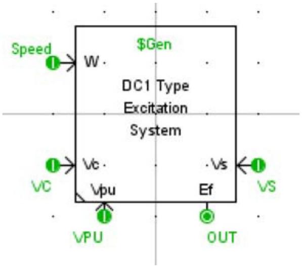 | |
| Figure 7.1:EXDC1 Component Icon | |
| The component icon for the exciter includes five I/O points. Four signal inputs and one signal output, all are real. | |
| Save the component builder icon to a new file name located in the RTDS_USER|ULIB folder. | |
| # 7.3 ADDINGTHEMODELCODE | |
| Select the 'C File Associations' tab. Select the $^{\prime \prime} + ^{\prime \prime}$ icon to Add New Association. Enter a model name. Input and Output points (listed under the IO Points tab) and user defined parameters (listed under the Parameters tab) are automatically associated with the model and placed in the .h file. Left clicking the "View Header File" button opens the .h file in an editor. The model includes four inputs, one output and a number of parameters: | |
| INPUTS: | |
| INPUTS:double VPU;double VS;double Speed;double VC; | |
| OUTPUTS: | |
| double OUT; | |
| # PARAMETERS: | |
| char Gen[11];int Mon;int PSS;double Vi;double Tr;double Ka;double Ta; | |
| # 7.4 SAMPLE C'CODE FOR THE DC1 TYPE EXCITER | |
| The C code is written for the model by clicking on the edit icon to open up the text editor window. The code for the DC1 type exciter is based on the block diagram shown in Figure 7.2. | |
| 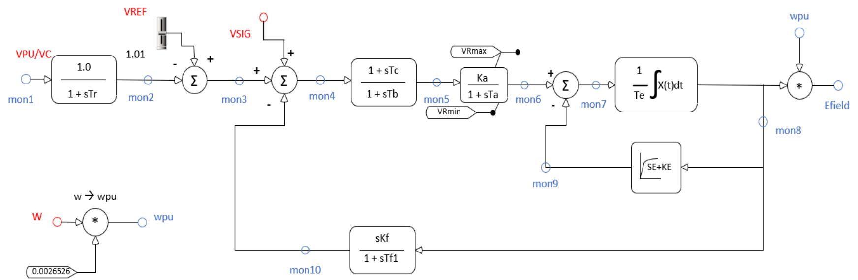 | |
| Figure 7.2: EXDC1 Diagram | |
| - The data preparation and code for the DC1 type exciter is shown below. VERSION: 3.001 #include "myEXDC1.h" | |
| STATIC: | |
| double dt,washoutG; double Vmax,Vref,tmp; double effoi,Verr,v_init; double mon1,mon2,mon3,mon4,mon5,mon6,mon7,mon8,mon9,mon10; int mon_array[10] $=$ {1,2,3,4,5,6,7,8,9,10}; | |
| include <builtin_gcc_generatorStructures.h> | |
| struct realpolex realpole1; struct realpolex realpole2; struct integratorx integrator1; struct washoutx washout1; struct leadlagx leadlag1; struct satKEx satKE1; | |
| RAM FUNCTIONS: | |
| include "initTransferFunctions.inc" | |
| RAM: | |
| dt= getTime- step(); | |
| # /\* Parameter Validation \*/ | |
| if(Vrmax $< = 0.0$ { | |
| if(E2<E1) { printf("\nWarning: Vrmax is less than zero."); printf("\n E2 must be greater than E1"); printf("\n Subsystem %d, Machine %s, exciter type EXDC1A.\n", getSubsystem(), Gen); reportError("EXDC1",1); } | |
| Vrmax = (Se2 + Ke)*E2; Vrmin = - 1\*Vrmax; } | |
| if (Vrmax < Vrmin) { tmp = Vrmin; Vrmin = Vrmax; Vrmax = tmp; printf("\nWarning: Vrmax is less than Vrmin."); printf("\n Vrmin set to Vrmax and Vrmax set to Vrmin"); printf("\n Subsystem %d, Machine %s, exciter type EXDC1. \n", getSubsystem(), Gen); reportError("EXDC1",1); } | |
| /* read initial field voltage */ efdli = get_data(Gen,"Efdli"); | |
| /* Compute initial Vrei value */ if (Vi < 0.0 || LFI $\mathsf{i} = =1$ { Vi= get_data(Gen,"Vpu"); if (LDComp == 1) { | |
| Vi = computeInitVcomp(Gen); } } | |
| /* Compute initial Se + KE */ if (Ke == 0.0) { v_init = 0.0; printf("\nWarning: Ke entered as 0.0. Calculation of Ke such that the"); printf("\n initial condition of Vc is zero is not supported."); printf("\n Subsystem %d, Machine %s, exciter type EXDC1. \n", getSubsystem(), Gen); reportError("EXDC1x", 1); } else { v_init = initSatKE(E1, Se1, E2, Se2, efldi, Ke, &satKE1); } printf("The value of v_init is %f\n", v_init); Verr = v_init / Ka; Vref = Verr + Vi; | |
| Vmax= 1.2; if (Vref > Vmax) Vmax= 1.2\*Vref; | |
| /* the create_slider function is in the .h file in the INPUTS section */ /* Initialize variables for real pole #1 */ initRealPole(1.0, 11, vi, vi, &realpole1); /* Initialize variables for lead - lag */ initLeadLag(Tb, Tc, Verr, Verr, &leadlag1); /* Initialize variables for real pole #2 */ initRealPole(Ka, Ta, Verr, v_init, &realpole2); /* Initialize variables for wash out */ | |
| washoutG = Kf/Tf1; initWashout(washoutG,Tf1,efldi,&washout1); /* Initialize variables for integrator */ initIntegrator(Te,0.0,efldi,&integrator1); | |
| # /* Check initial output values are within Vrmax and Vrmin limits */ | |
| if (v_init > Vrmax || v_init < Vrmin) { printf("\nWarning: Initial value of mon6 is not within the entered limits."); printf("\n VRmax = %f, VRmin = %f, mon6 initial value = %f.", Vrmax, Vrmin, v_init); printf("\n Subsystem %d, Machine %s, exciter type EXDC1x.\n", getSubsystem(), Gen); reportError("EXDC1x", 1); } | |
| /* Initialize all monitoring variables that are going to be referenced in the code section before they are assigned a value */ | |
| mon9 = v_init; mon10 = 0.0; | |
| CODE: | |
| double puSpeed; | |
| # /* Include load compensation */ | |
| if (LDComp==1) | |
| { mon1 = VC; } else | |
| } else | |
| else | |
| { | |
| mon1 = VPU; } | |
| /* realpole #1 */ | |
| mon2 = realPole(mon1, 1.0, 0, 0.0, 0.0, 0.0, 0.0, &realpole1); | |
| /\* Summing junction \*/ mon3 $=$ Vref1- mon2; /\* Optionally include stabilizer input \*/ if $(\mathsf{PSS} = =1)$ { mon3 $=$ mon3+VS; } mon4 $=$ mon3- mon10; /\* lead- lag \*/ mon5 $=$ leadLag(mon4,1.0,0.0,0.0,0.0,0.0,&leadlag1); /\* realpole #2 \*/ mon6 $=$ realPole(mon5,Ka,1,Vrmin,Vrmax,0,0,0.0,&realpole2); /\* Summing Junction \*/ mon7 $=$ mon6- mon9; /\* Integrator \*/ mon8 $=$ integrator(mon7,0,0.0,0.0,0,0.0,0.0,&integrator1); /\* Saturation Function \*/ mon9 $=$ satKE(mon8,&satKE1); | |
| /\* Washout \*/ mon10 $=$ washOut(mon8,washoutG,0,0.0,0.0,0.0,0.0,&washout1); | |
| /\* Efd \*/ OUT $=$ mon8; if (spdMult $= = 1$ { puSpeed $=$ Speed/wBase; OUT $=$ mon8 \* puSpeed; } | |
| # /check if monitoring is enabled, if so assign the output based on the dial position\*/ | |
| if (Mon $= = 1$ { if (dial1 $= = 2$ { internalV $=$ mon2; } else if (dial1 $= = 3$ { internalV $=$ mon3; } else if (dial1 $= = 4$ { internalV $=$ mon4; } else if (dial1 $= = 5$ { internalV $=$ mon5; } else if (dial1 $= = 6$ { internalV $=$ mon6; } else if (dial1 $= = 7$ { internalV $=$ mon7; } else if (dial1 $= = 8$ { internalV $=$ mon8; } | |
| else if (dial1 == 9) { internalV = mon9; } else if (dial1 == 10) { internalV = mon10; } else { internalV = mon1; } | |
| # 7.5 DATA PREPARATION AND INITIALIZATION | |
| Generic generator control models include the capability to initialize their internal variables and to configure set- point sliders. Given the initial field voltage, the initial terminal voltage and various gains of the exciter components, it is possible to compute the initial inputs and output associated with each block of the DC1 controller. The initial terminal voltage and gains of the exciter components are entered to the component as parameters. The initial field voltage is computed by the generator model code and can be accessed using the get_data function. The get_data function locates and returns data from another component. In the RAM section the initial field voltage is determined using the code below; | |
| $$ | |
| \mathsf{e}\mathsf{f}\mathsf{I}\mathsf{d}\mathsf{i} = \mathsf{g}\mathsf{e}\mathsf{t}\_ \mathsf{data}(\mathsf{Gen},\mathsf{"E}\mathsf{f}\mathsf{I}\mathsf{d}\mathsf{i}^{\prime \prime}); | |
| $$ | |
| The get data function requires two arguments. The first argument is the name of the component, the second argument is the parameter name. | |
| The name of the generator to which the exciter model is connected is required as a parameter named 'Gen'. | |
| The generator model pre- calculates the field voltage required to provide the desired real and reactive power output. This data is written to the .map file and given the variable "Efdi". To extract the initial field voltage from the generator model, the parameter name Efdi must be passed to the get_data function. The parameter name is case sensitive. | |
| The error is calculated as the initial output of the saturation block 'v_init' divided by the gain Ka. | |
| Verr $=$ v_init/Ka; | |
| The initial value for Vref slider is computed as: | |
| Vref $=$ Vi $^+$ Verr; Vmax $=$ 1.2; if Vref $\gnsim$ Vmax Vmax $=$ 1.2\*(Vref); | |
| The initial value 'Vref' and the maximum value 'Vmax' are used to initialize the slider in the following section 'ADD AN INTERNAL SLIDER'. | |
| Commonly used control functions are available as function calls in CBuilder. In this case, the realPole, leadLag, washOut and Integrator functions are used. To use these functions in the CODE section, the history terms must first be initialized in the RAM section. The calculated history terms are then stored in a structure for use within the CODE section. The initialization functions are stored in a file named "initTransferFunctions.inc". This include statement must appear in the RAM FUNCTIONS section. Optionally, the initialization functions could appear directly in the RAM FUNCTIONS section and not in an include file. Please see APPENDIX E of the CBuilder User's Manual for complete details on initialization of the transfer functions. | |
| RAM FUNCTIONS: | |
| include "initTransferFunctions.inc" | |
| The functions in the 'initTransferFunctions.inc' file can be called from the RAM section. | |
| /\* Initialize variables for saturation function \*/ if $(\mathtt{Ke}< = 0.0)$ { v_init $=$ initSatKE0(E1,Se1,E2,Se2,efldi,Vrmax,Cal,&satKE1); } else { v_init $=$ initSatKE(E1,Se1,E2,Se2,efldi,Ke,Cal,&satKE1); } | |
| /\* Initialize variables for real pole #1 \*/ initRealPole(1.0,Tr,Vi,Vi,&realpole1); /\* Initialize variables for lead - lag \*/ initLeadLag(Tb,Tc,Verr,Verr,&leadlag1); /\* Initialize variables for real pole #2 \*/ | |
| initRealPole(Ka,Ta,Verr,v_init,&realpole2); /\* Initialize variables for wash out \*/ washoutG $=$ Kf/Tf1; initWashout(washoutG,Tf1,efldi,&washout1); /\* Initialize variables for integrator $\neq \neq$ initIntegrator(Te,0.0,efldi,&integrator1); | |
| For example, to initialize the first realpole, the gain, time constant, initial input, initial output and realpole structure are passed as parameters. The initial input and output of the realpole are set to initial p.u voltage of the generator. The leadLag is initialized next, the precalculated Verr value is passed as the initial input and output of the leadlag. | |
| # 7.6 ADD AN INTERNAL SLIDER | |
| Referring to the block diagram, a slider Vref is required as input to the control block. The slider is an internal input to the component meaning that a physical input connection does not exist on the component. | |
| Add an internal slider. Click the Add Variable button (see 1 of Figure 7.3) and then select SLIDERS from the Section drop down menu in the "Add Variable" window (see 2 of Figure 7.3). | |
| 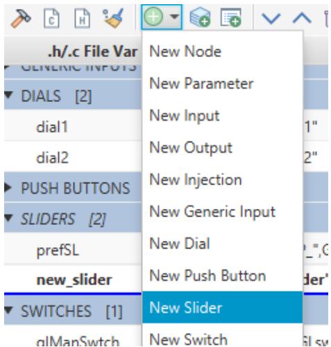 | |
| Figure 7.3: Adding an Internal Slider | |
| When the parameter is selected the edit menu appears to the right window as shown in Figure 7.4. | |
| 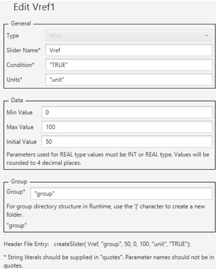 | |
| Figure 7.4: Slider Menu Edit Option | |
| - Assign a variable name to the slider so it can be referenced in the Code section. In this example Vref1 is used. | |
| - A slider name is required. This is the name of the slider as it will appear in RunTime. To duplicate existing generic generator control models the Vref slider is located under the CTLs|Inputs group and named V_generator name. To concatenate two strings together, the strcat2 function can be used to create the slider name. The initial value of the slider has been calculated in the RAM section and assigned to variable Vref. The maximum value of the slider has also been calculated in the RAVI section and assigned to variable Vmax. The variables Vref and Vmax are entered as Initial Value and Max Value. | |
| - Save the CBuilder component. | |
| After saving the component, a create_slider function appears in the INPUTS: section of the .h file. The slider name 'Vref1' can be used within the CODE section of the .c file. | |
| # 7.7 ADD CODE FOR REALPOLE FUNCTION | |
| The function realPole implements the transfer function as shown in Equation 7- 1. | |
| $$ | |
| Y(s) = \frac{G}{(1 + sT)} *X(s) | |
| $$ | |
| Equation 7- 1 | |
| In the code section, the realPole function is called as follows: | |
| # /\* realpole \*/ | |
| out $\equiv$ realPole(Input, Gain, Limit, minLim, maxLim,RST,RSTSIG,RVAL, &realpole1); | |
| The realPole function requires nine arguments. For a complete description of the arguments please see APPENDIX E of the CBuilder User's Manual. The function returns the output Y(s) of the realpole transfer function. | |
| # 7.8 ADD CODE LEADLAG FUNCTION | |
| The function leadLag implements the transfer function as shown in Equation 7- 2. | |
| $$ | |
| Y(s) = \frac{G(1 + sT1)}{(1 + sT2)} *X(s) | |
| $$ | |
| Equation 7- 2 | |
| In the code section, the leadLag function is called as follows: | |
| # /\* leadLag \*/ | |
| out $\equiv$ leadLag(Input, Gain, Limit, minLim, maxLim,RST,RSTSIG,RVAL, &leadlag1); | |
| The leadLag function requires nine arguments. For a complete description of the arguments please see APPENDIX E of the CBuilder User's Manual. The function returns the output Y(s) of the leadLag transfer function. | |
| # 7.9 ADD CODE FOR WASHOUT FUNCTION | |
| The function washOut implements the transfer function as shown in Equation 7- 3. | |
| $$ | |
| Y(s) = \frac{GsT}{(1 + sT)} *X(s) | |
| $$ | |
| Equation 7- 3 | |
| In the code section, the washOut function is called as follows: | |
| # /\* washOut\*/ | |
| out $\equiv$ washOut(Input, Gain, Limit, minLim, maxLim,RST,RSTSIG,RVAL, &washout1); | |
| The washOut function requires nine arguments. For a complete description of the arguments please see APPENDIX E of the CBuilder User's Manual. The function returns the output Y(s) of the washOut transfer function. | |
| # 7.10 ADD CODE FOR SATURATION FUNCTION | |
| The saturation function satKE implements the saturation curve. | |
| 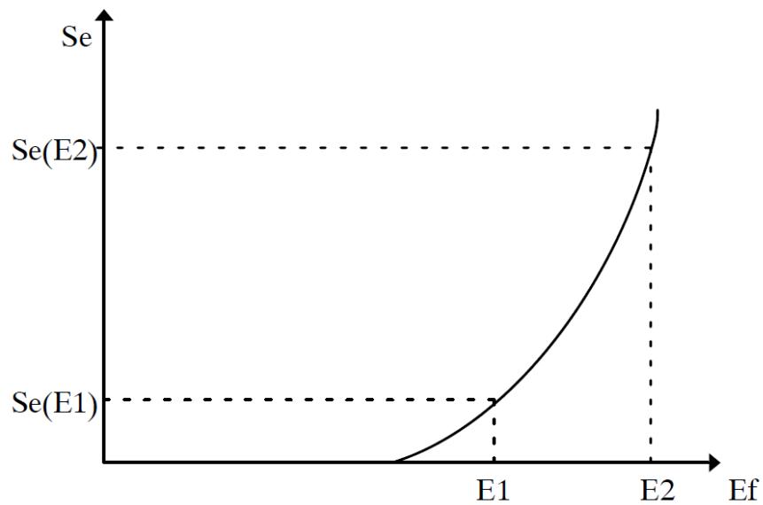 | |
| Figure 7.5: Saturation Curve | |
| In the code section, the satKE function is called as follows: | |
| /\* saturation \*/ out $\equiv$ satKE(Input, &satKE1); | |
| # 7.11 ADDING THE CODE | |
| Read in the p.u. voltage and check for load compensation. | |
| if $\scriptstyle (\mathtt{LDComp} = =1)$ { monl $=$ VC; } else { monl $=$ VPU} | |
| Add function call for the first realpole function. | |
| mon2 $=$ realPole(VPU, 1.0, 0, 0.0, 0.0, 0.0, 0.0, 0.0, &realpole1); | |
| The realpole function requires nine arguments. The first argument is the input. Input to the first realpole block is the p.u. voltage from the generator model. This input is | |
| an I/O point on the component and declared in the .h file as VPU. | |
| The second argument is the gain. The gain is fixed at 1.0. | |
| The third, fourth and fifth arguments are for limits. Limits are not included in this block and therefore set to 0. | |
| The sixth, seventh and eighth arguments are for reset. Reset is not included in this block and therefore set to 0. | |
| The ninth argument is the realpole structure. The variables within the structure were initialized in the RAM section. | |
| The output from the realpole is assigned the variable name 'mon2' according to the block diagram. | |
| Add code for the summing junction. | |
| /\* Summing junction \*/ | |
| mon3 $=$ Vref1 - mon2; | |
| /\* Optionally include stabilizer input \*/ | |
| if $\mathrm{PSS} = =1$ | |
| { mon3 $=$ mon3 $^+$ VS; } | |
| The summing junction subtracts the output from the realpole 'mon2' from the Vref slider. An optional third input can exist to the summing junction. If the parameter PSS is set to YES in the component, a stabilizer input signal input is available and added to the above. The output from the summing junction is assigned the variable name mon3. | |
| Add code for the summing junction. | |
| $$ | |
| \mathrm{mon4} = \mathrm{mon3} - \mathrm{mon10}; | |
| $$ | |
| The output from the washout block (mon10) is subtracted from the output of the previous summing junction according to the block diagram. | |
| Add function call for the leadlag function. | |
| mon5 $=$ leadLag(mon4,1.0,0,0.0,0.0,0,0.0,&leadlag1); | |
| The leadLag function requires nine arguments. The first argument is the input. Input to the leadLag function is the output from the previous summing junction (mon4). | |
| The second argument is the gain. The gain is fixed at 1.0. The third, fourth and fifth arguments are for limits. Limits are not included in this block and therefore set to 0. | |
| The sixth, seven and eighth arguments are for reset. Reset is not included in this block and therefore set to 0. | |
| The ninth argument is the leadlag structure. The variables within the structure were initialized in the RAM section. | |
| The output from the leadlag is assigned the variable name 'mon5' according to the block diagram. | |
| Add function call for the second realpole function. | |
| mon6 = realPole(mon5, Ka, 1, Vrmin, Vrmax, 0, 0, 0.0, &realpole2); | |
| Input to the second realPole function is the output from the leadlag (mon5). | |
| The second argument is the gain. The gain 'Ka' is entered as a parameter. | |
| Limits are included in the second realPole, therefore the third argument is set to 1. | |
| The fourth and fifth arguments are the minimum and maximum limits Vrmin and Vrmax. Vrmin and Vrmax are parameters entered by the user. | |
| The sixth, seven and eighth arguments are for reset. Reset is not included in this block and therefore set to 0. | |
| The ninth argument is the realpole#2 structure. The variables within the structure were initialized in the RAM section. | |
| The output from the realpole is assigned the variable name mon6 according to the block diagram. | |
| Add code for summing junction. | |
| $$ | |
| \mathtt{mon7} = \mathtt{mon6} - \mathtt{mon9}; | |
| $$ | |
| The output from the saturation block (mon9) is subtracted from the output of realpole#2 (mon6). | |
| Add function call for the integrator function. | |
| mon8 = integrator(mon7, 0, 0.0, 0.0, 0.0, 0.0, &integrator1); | |
| The first argument in the integrator function call is the input. Input to the integrator function is the output from the previous summing junction (mon7). | |
| The second, third and fourth arguments are for limits. Limits are not included in this block and therefore set to 0. | |
| The fifth, sixth and seven arguments are for reset. Reset is not included in this block and therefore set to 0. | |
| The eighth argument is the integrator structure. The variables within the structure were initialized in the RAM section. | |
| The output from the integrator is assigned the variable name 'mon8' according to the block diagram. | |
| Add function call for the saturation function. | |
| $$ | |
| \mathsf{mon9} = \mathsf{satKE}(\mathsf{mon8},\& \mathsf{satKE}); | |
| $$ | |
| The first argument in the satKE function call is the input. Input to the satKE function is the output from the previous integrator (mon8). | |
| The second argument is the saturation structure. The variables within the structure were initialized in the RAM section. | |
| Add function call for the washout function. | |
| mon10 = washOut(mon8, washoutG, 0.0, 0.0, 0.0, 0.0, &integrator); | |
| The first argument in the washOut function call is the input. Input to the washOut function is the output from the integrator (mon8). | |
| The second argument is the gain. The gain is computed as Kf/1f1. | |
| The third, fourth and fifth arguments are for limits. Limits are not included in this block and therefore set to 0. | |
| The sixth, seventh and eighth arguments are for reset. Reset is not included in this block and therefore set to 0. | |
| The ninth argument is the washout structure. The variables within the structure were initialized in the RAM section. | |
| The output from the washout is assigned the variable name 'mon10' according to the block diagram. | |
| Add multiplier and compute the output field voltage. | |
| if (spDMult == 1) { puSpeed = Speed/wBase; OUT = mon8 * puSpeed; } | |
| The p.u speed is determined by dividing the machine speed by the base value (wBase). wBase is a parameter entered by the user and Speed is an I/O point on the component and declared in the .h file as Speed. | |
| The output from the integrator (mon8) is multiplied by the p.u. speed of the machine to produce the field voltage (OUT). The signal OUT is an I/O point on the component and declared in the .h file as OUT. | |
| # 7.12 ADD A DIAL TO SELECT INTERNAL VARIABLES FOR MONITORING | |
| Internal variables are displayed on the block diagram of the DC1 controller and are identified with a mon# wire label. To maintain similar operation to existing generator controls, only one internal variable may be monitored at one time in RunTime. The position of a dial indicates which internal variable is displayed in RunTime. | |
| - Add an internal dial. Click the Add Variable button (see 1 of Figure 7.6) and then select DIALS from the Section drop down menu in the "Add Variable" window (see 2 of Figure 7.6). | |
| 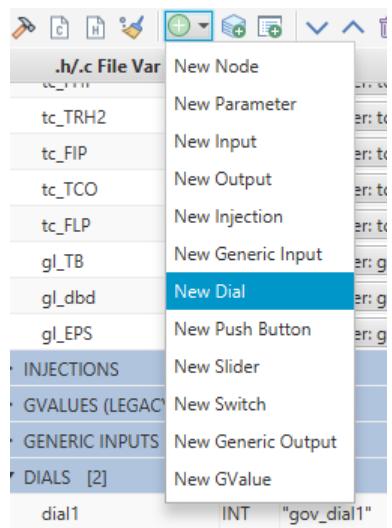 | |
| Figure 7.6: Adding a Dial | |
| - Assign a variable name to the dial so it can be referenced in the Code section. In this example dial1 is used. | |
| - Use the Edit dial window to enter initial values for the dial. | |
| - A dial name is required. This is the name of the dial as it will appear in RunTime. To duplicate existing generic generator control models the dial is named "exc_mon" and is located under the Machines|generatørname group to concatenate two strings together, the strcat2 function can be used to create the Group name. The number of internal monitoring variables is 10, therefore the number of positions available on the dial has been set to 10. The initial position of the dial is set to 1. The dial values are stored in an array with name mon_array. This array must be declared in the static section of the .c file. Creation of the dial is conditional. If the parameter Mon | |
| (Monitor internal variable) is toggled to Yes, then the dial is created. | |
| Save the CBuilder component. | |
| After saving the component, a create_dial function appears in the INPUTS: section of the .h file. The dial name 'dial1' can be used within the CODE section of the .c file. | |
| # 7.13 ADD A GENERIC OUTPUT | |
| An output signal must be added to display the monitored internal variable in RunTime. | |
| Add a generic output variable. | |
| 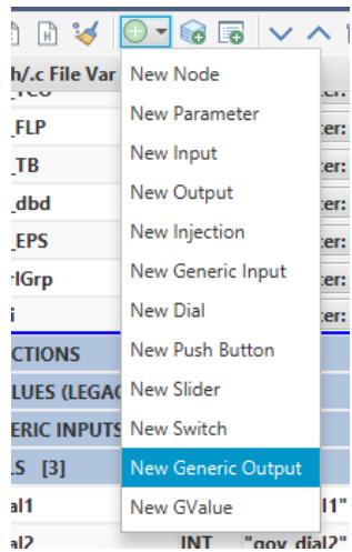 | |
| Figure 7.7: Adding a Generic Output | |
| Assign a variable name to the generic output so it can be referenced in the Code section. In this example internalV is used. | |
| Use edit option to enter the initial values for the generic output variable. | |
| A generic output is required to display internal variables in RunTime. An output name is required, this is the name of the signal as it will appear in RunTime. The variable name ivName is entered. 'ivName' is a parameter. Therefore, the signal name entered as parameter 'ivName' is used as the output name. To duplicate existing generic generator control models, the signal name is located under the Machines|generatorname group. To concatenate two strings together, the strcat2 function can be used to create the Group name. Creation of the generic output is conditional. If the parameter Mon (Monitor internal variable) is toggled to Yes, then the output signal is created. | |
| # 7.14 ADD MONITORING CODE | |
| The internal variables named mon# can be plotted in RunTime. The signal to monitor is based | |
| on the dial position. | |
| Add monitoring code for internal variables. | |
| if $(\mathtt{Mon} = = 1)$ { if (dial1 == 2) { internalv $=$ mon2; } else if (dial1 == 3) { internalv $=$ mon3; } else if (dial1 == 4) { internalv $=$ mon4; } else if (dial1 == 5) { internalv $=$ mon5; } else if (dial1== 6) { internalv $=$ mon6; } else if (dial1 == 7) { internalv $=$ mon7; } else if (dial1 == 8) { internalv $=$ mon8; } else if (dial1==9) { | |
| internalV $=$ mon9; } else if (dial1 $\scriptstyle = = 10$ { internalV $=$ mon10; } else { internalV $=$ monl; } } | |
| Monitoring is enabled if the parameter Mon is toggled to Yes in the component. If the dial position is 2, then the generic output signal 'exc_mon1' is assigned internal variable mon2. If the dial position is 3, then the generic output signal 'exc_mon1' is assigned internal variable mon3 etc. This code continues until all 9 dial positions have been associated with an output. Note: the variable name of the dial declared in the .h file is dial1. The dial name in RunTime will appear as exc_dial. The variable name of the generic output declared in the .h file is exc_mon1. The name of the generic output will appear in RunTime as exc_mon. | |
| # 8 SIMPLE TRANSFORMER | |
| # 8.1 INTRODUCTION | |
| 8.1 INTRODUCTIONThe transformer model developed in this tutorial will include winding resistance, leakage reactance as well as a linear magnetizing reactance. The effect of core saturation will not be considered. | |
| # 8.2 THEORY | |
| # 8.2.1 Modelling a Transformer | |
| 8.2 THEORY8.2.1 Modelling a TransformerMost power system components, regardless of their complexity, are simplified so that they are modeled as one or more current sources in parallel with a conductance. The difficulty in modeling components is often a problem of finding such a representation that accurately represents the physical properties of the device being modeled. Our goal is to reduce the two- winding transformer to something similar to what is shown in Figure 8.1. The equations developed must model the coupling between the two windings of the transformer. | |
| 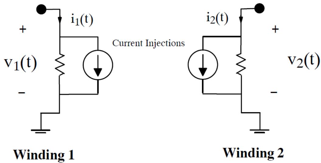 | |
| Figure 8.1: Framework for How to Model a Transformer | |
| One of the keys to writing a successful power system model is to write out the correct equations. It may be possible to write a set of equations in the continuous time- domain which accurately represent the behavior of a particular piece of equipment but it may not | |
| be possible to discretize these equations in such a way that they can be seamlessly integrated with the RTDS Solution Algorithm. Not only must the equations written be correct in terms of physics, they must also integrate into the existing solution framework of the simulator. The selection of the proper equations is often dependent upon experience. | |
| Consider the per- unitized equivalent circuit for a transformer given in Figure 8.2. The winding resistance and leakage reactance have been divided in half and the magnetizing branch has been connected in the middle. Two loop equations can be written for this circuit. The resulting equations are given by Equation 8- 1 and Equation 8- 2. | |
| 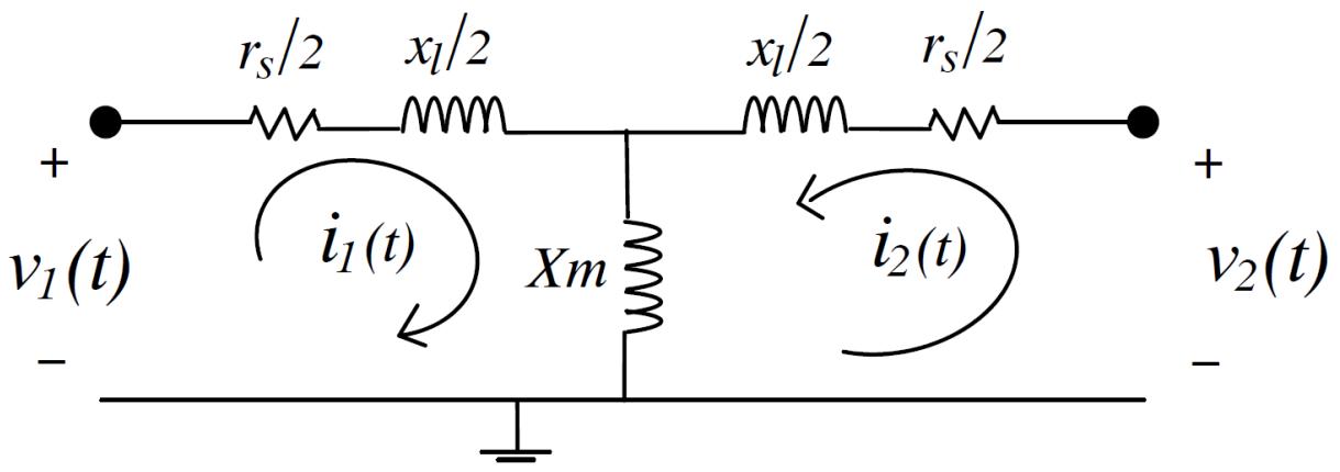 | |
| Figure 8.2: Per-Unitized Equivalent Circuit for a Transformer | |
| $$ | |
| v_{1}(t) = \frac{rs}{2} i_{1}(t) + j\frac{x_{l}}{2} i_{1} + jx_{m}\big(i_{1}(t) + i_{2}(t)\big) | |
| $$ | |
| $$ | |
| v_{2}(t) = \frac{rs}{2} i_{2}(t) + j\frac{x_{l}}{2} i_{2}(t) + jx_{m}\big(i_{1}(t) + i_{2}(t)\big) | |
| $$ | |
| Equation 8- 1 | |
| Equation 8- 2 | |
| The values in Equation 8- 1 and Equation 8- 2 are all per- unitized; Equation 8- 1 and Equation 8- 2 are re- written in ohmic values as Equation 8- 3 and Equation 8- 4, respectively. Equation 8- 3 has been referred to the primary side while Equation 8- 4 has been referred to the secondary side. | |
| $$ | |
| v_{1}(t) = \frac{rs}{2}\frac{v_{rated}}{s_{rated}} i_{1}(t) + j\left(\frac{x_{l}}{2} +x_{m}\right)\frac{v_{rated}}{s_{rated}} i_{1}(t) + jx_{m}\frac{v_{rated}}{s_{rated}}\frac{v_{rated}}{v_{rated}} i_{2}(t) | |
| $$ | |
| Equation 8- 3 | |
| $$ | |
| v_{2}(t) = \frac{rs}{2}\frac{v_{rated}}{s_{rated}} i_{2}(t) + j\left(\frac{x_{l}}{2} +x_{m}\right)\frac{v_{rated}}{s_{rated}} i_{2}(t) + jx_{m}\frac{v_{rated}}{s_{rated}}\frac{v_{rated}}{v_{rated}} i_{1}(t) | |
| $$ | |
| Equation 8- 4 | |
| Written in matrix form, Equation 8- 3 and Equation 8- 4 become Equation 8- 5 and Equation 8- 6, respectively. | |
| $$ | |
| \begin{array}{r l} & {[v_{1}(t)] = \frac{1}{s_{r a t e d}}[[ \begin{array}{c c}{\frac{r_{s}}{2} v_{r a t e d_{1}}^{2}} & 0\\ 0 & {\frac{r_{s}}{2} v_{r a t e d_{2}}^{2}} \end{array} ]}\\ & {\qquad +j[ \begin{array}{c c}{(x_{m} + \frac{x_{l}}{2})v_{r a t e d_{1}}^{2}} & {x_{m}v_{r a t e d1}v_{r a t e d2}}\\ {x_{m}v_{r a t e d1}v_{r a t e d2}} & {(x_{m} + \frac{x_{l}}{2})v_{r a t e d_{2}}^{2}} \end{array} ]][ \begin{array}{c}{i_{1}(t)}\\ {i_{2}(t)} \end{array} ]} \end{array} | |
| $$ | |
| Equation 8- 5 | |
| $$ | |
| \left[ \begin{array}{c}v_{1}(t)\\ v_{2}(t) \end{array} \right] = \left[r\right]\left[ \begin{array}{c}i_{1}(t)\\ i_{2}(t) \end{array} \right] + j\left[l\right]\left[ \begin{array}{c}i_{1}(t)\\ i_{2}(t) \end{array} \right] | |
| $$ | |
| Equation 8- 6 | |
| Equation 8- 6 can be converted from the Laplace domain into the time domain and yields Equation 8- 7. | |
| $$ | |
| \left[ \begin{array}{c}v_{1}(t)\\ v_{2}(t) \end{array} \right] = \left[r\right]\left[ \begin{array}{c}i_{1}(t)\\ i_{2}(t) \end{array} \right] + \left[l\right]\left[ \begin{array}{c}\frac{\delta i_{1}(t)}{\delta t}\\ \frac{\delta i_{2}(t)}{\delta t} \end{array} \right] | |
| $$ | |
| $$ | |
| [v(t)] = [r][i(t)] + [l]\left[\frac{\delta i(t)}{\delta t}\right] | |
| $$ | |
| Equation 8- 8 | |
| Equation 8- 8 can then be numerically integrated over a time- step using trapezoidal integration. | |
| $$ | |
| \left[\frac{\left(v(t) + v(t - \Delta t)\right)}{2}\Delta t\right] = [r]\left[\frac{(i(t) + i(t - \Delta t))}{2}\Delta t\right] + [l][i(t) - i(t - \Delta t)] | |
| $$ | |
| Equation 8- 9 | |
| Reorganization of Equation 8- 9 leads to Equation 8- 10. | |
| $$ | |
| [i(t)] = [g_{Tr}][v(t)] + [ih(t)] | |
| $$ | |
| Equation 8- 10 | |
| Where: | |
| $$ | |
| g_{Tr} = \Delta \frac{t}{2}\left[\frac{[r]\Delta t}{2} +[l]\right]^{-1} | |
| $$ | |
| Equation 8- 11 | |
| $$ | |
| \left[ih(t)\right] = \left[g_{Tr}\right]\left[[v(t - \Delta t)] - \left[[r] - [l]\frac{2}{\Delta t}\right][i(t - \Delta t)]\right] | |
| $$ | |
| Equation 8- 12 | |
| Equation 8- 10 describes the currents entering the two terminals of the transformer. Each of these two currents has two components. A portion of each current is a function of the voltages across the terminals of the transformer at the current time- step. The other portion | |
| of each current can be considered as being contributed by a current source that is a function strictly of the currents flowing into the transformer and the voltages across the terminals of the transformer at the previous time- step. The component of the current vector $[i(t)]$ that is a function of past voltages and currents is grouped and labeled as $[ih(t)]$ . This term is generally known as a history current because it is a function strictly of the past voltages and currents across and through the transformer. | |
| At this point it is instructive to take a step back and look at the RTDS Simulator's algorithm in order to show how Equation 8- 10 can be incorporated into it. | |
| # 8.2.2 RTDS Solution Algorithm | |
| The most effective way to explain the RTDS Solution Algorithm is to do so via example. Figure 8.3 shows a simple source connected to an RLC circuit. Two nodes have been labeled. | |
| 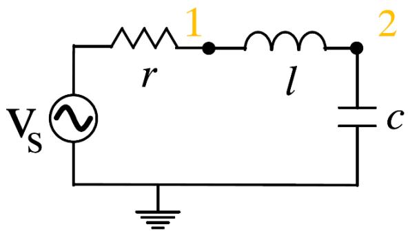 | |
| Figure 8.3: Arbitrary Circuit Used to Demonstrate RTDS Solution Algorithm | |
| A Norton equivalent can be found for the voltage source and series resistance. It can be shown that both the inductor and capacitor can each be represented by a current source in parallel with a conductance. [1] The current sources become functions of past voltages and currents across and through the element and are generally referred to as history currents. For this tutorial the details of how to calculate these history currents is not critical; assume they are known quantities. An equivalent for Figure 8.3 can then be drawn as shown in Figure 8.4. The circuit now consists strictly of current sources and conductance. | |
| 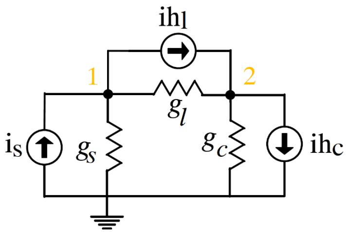 | |
| Figure 8.4: Arbitrary Circuit Modified so that it Consists Purely of Current Sources and Conductance Values | |
| Writing the nodal equations at nodes 1 and 2 leads to Equation 8- 13 and Equation 8- 14 which can be written in matrix form as shown in Equation 8- 15. | |
| $$ | |
| \begin{array}{c}{i_s = ih_l + v_1\cdot g_s + (v_1 - v_2)\cdot g_l}\\ {}\\ {ih_l = ih_c + (v_2 - v_1)\cdot g_l + v_2\cdot g_c}\\ {}\\ {[g_s + g_l\qquad -g_l\qquad ][v_1] = [i_s - ih_1]}\\ {}\\ {-g_l\qquad g_l + g_c][v_2] = [ih_1 - ih_c]} \end{array} \tag{Equation 8-13} | |
| $$ | |
| In Section 8.2.3 the calculations needed to simulate the interconnected circuits of this and the previous section are enumerated. Details about how these calculations are divided among several processors are then given. | |
| # 8.2.3 Integrating the Transformer Model into the RTDS Solution Algorithm | |
| In the circuit of Figure 8.5 the simple transformer model has been added to the arbitrary circuit of Figure 8.4. The nodal equations for this circuit can be written as before except now our system has three nodes. The resulting equations are shown in Equation 8- 16, Equation 8- 17, and Equation 8- 18. | |
| 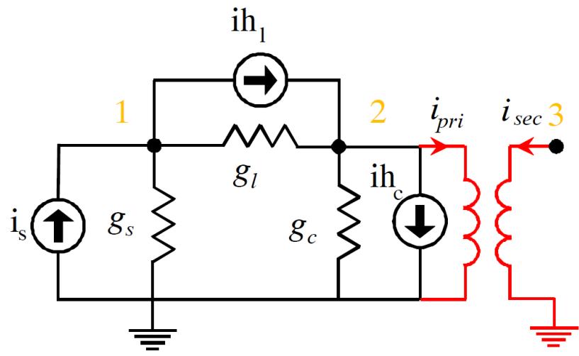 | |
| Figure 8.5: Arbitrary Circuit with Simple Transformer Added to it | |
| $$ | |
| i_{s} = ih_{1} + v_{1}\cdot g_{s} + (v_{1} - v_{2})\cdot g_{l} | |
| $$ | |
| Equation 8- 16 | |
| $$ | |
| ih_{l} = ih_{c} + (v_{2} - v_{1})\cdot g_{l} + v_{2}\cdot g_{c} + i_{pri} | |
| $$ | |
| Equation 8- 17 | |
| $$ | |
| 0 = i_{sec} | |
| $$ | |
| Equation 8- 18 | |
| if Equation 8- 10 is rewritten with the appropriate indexing the terms ipri and isec can be defined as given in the following equation. | |
| $$ | |
| \begin{array}{r}\left[ \begin{array}{c}i_{pri}\\ i_{sec} \end{array} \right] = \left[ \begin{array}{cc}g_{TR22} & g_{TR23}\\ g_{TR32} & g_{TR33} \end{array} \right]\left[ \begin{array}{c}v_{2}\\ v_{3} \end{array} \right] + \left[ \begin{array}{c}ih_{pri}\\ ih_{sec} \end{array} \right] \end{array} | |
| $$ | |
| Equation 8- 19 | |
| Substituting Equation 8- 19 into Equation 8- 16, Equation 8- 17, and Equation 8- 18 and re- arranging them gives the matrix Equation 8- 20. | |
| $$ | |
| \left[ \begin{array}{ccc}{g_s + g_l} & {-g_l} & 0\\ {-g_l} & {g_l + g_c + g_{TR22}} & {g_{TR23}}\\ {0} & {g_{TR32}} & {g_{TR33}} \end{array} \right]\left[ \begin{array}{c}{v_1}\\ {v_2}\\ {v_3} \end{array} \right] = \left[ \begin{array}{c}{i_s - ih_l}\\ {ih_l - ih_c - ih_{pri}}\\ {-ih_{sec}} \end{array} \right] | |
| $$ | |
| Equation 8- 20 | |
| The solution to Equation 8- 20 is the solution of the circuit of Figure 8.5. Notice that this matrix can be assembled by inspection if parts of Equation 8- 15 and 8- 19 are 'overlayed' while using the appropriate indexing. | |
| Assuming the objective is to solve Equation 8- 20 for all the node voltages, the vector $[\mathsf{v}_1,\mathsf{v}_2,\mathsf{v}_3]^{\mathsf{T}}$ can be found by inverting the conductance matrix of Equation 8- 20. This leads to Equation 8- 21; time indices have been added for completeness. | |
| $$ | |
| \begin{array}{r}\left[ \begin{array}{c}v_{1}(t)\\ v_{2}(t)\\ v_{3}(t) \end{array} \right] = \left[ \begin{array}{ccc}g_{s} + g_{l} & -g_{l} & 0\\ -g_{l} & g_{l} + g_{c} + g_{TR22} & g_{TR23}\\ 0 & g_{TR32} & g_{TR33} \end{array} \right]^{-1}\left[ \begin{array}{c}i_{s}(t) - ih_{l}(t)\\ ih_{l}(t) - ih_{c}(t) - ih_{pri}(t)\\ -ih_{sec}(t) \end{array} \right] \end{array} | |
| $$ | |
| Equation 8- 21 | |
| Matrix Equation 8- 21 is representative of the main calculation completed by the RTDS Network Solution. It describes the interaction of all the elements in a circuit. | |
| Before the RHS of this equation can be calculated, the currents $i_{s}(t), i_{h}(t), i_{c}(t), i_{h_{c}}(t)$ and $i_{h_{sec}}(t)$ must be known. This is where the simulation gets broken up into several parts. | |
| The currents $i_{s}(t), i_{h_{pri}}(t)$ and $i_{h_{sec}}(t)$ which originate from the voltage source and transformer can be calculated in parallel on different processors in order to reduce the computation time. These current contributions will be referred to as current injections because they are injected into the RTDS Network Solution. | |
| The currents $ih_{s}(t)$ and $ih_{c}(t)$ are contributions from the circuit's inductor and capacitor. In general, the calculations associated with passive RLC components are included as part of the network solution. | |
| Figure 8.6 illustrates how the calculation of Equation 8- 21 is divided among several processors and gives some details about how the simple transformer model interacts with the Network Solution. Figure 8.6 is very simplified and many details have been omitted. | |
| 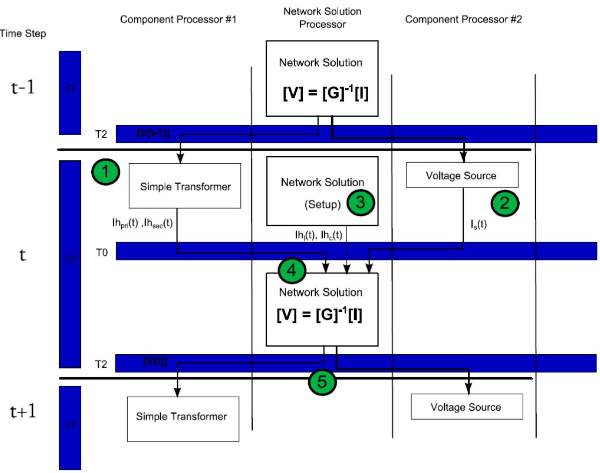 | |
| Figure 8.6: Interaction between Simple Transformer and the Network Solution | |
| 1. In the first part of any given time step, the network voltage vector from the previous time-step, [V(t-1)], are used to calculate the currents flowing into the transformer at the previous time-step, $i_{pri}(t - 1)$ and $i_{sec}(t - 1)$ . These two quantities can then be used to calculate the history currents for the transformer, $ih_{pri}(t - 1)$ and $ih_{sec}(t - 1)$ , using Equation 8-12. The calculations are done on a dedicated processor labeled component processor #1. | |
| 2. While the history currents are being calculated for the simple transformer on component processor #1, the calculation of $i_{s}(t - 1)$ for the voltage source are completed on a different processor labeled component processor #2. Details of the calculation of $i_{s}(t - 1)$ are not the focus of this tutorial. If the example circuit contained additional components like a generator or a transmission line the currents associated with those components could be calculated simultaneously on other processors in order to reduce the computation time. | |
| 3. The RTDS Network solution is responsible for the calculations associated with most passive RLC components so it calculates $\mathrm{ih}(t - 1)$ and $\mathrm{ih}_{\mathrm{c}}(t - 1)$ . | |
| 4. The currents calculated in (1)-(3) become the current injections for then network solution. The current injections are sent to the processor which calculates the main network solution at a designated time labeled communication interval $T0$ . The network solution then uses the current injections to calculate the circuit's node voltages by solving Equation 8-21. | |
| 5. The calculated voltages are passed to all the component processors and the process starts again at the next time-step. | |
| These five steps illustrate how the calculation of Equation 8- 21 could be divided among several processors on the RTDS Simulator. The simple transformer model that will be assembled in CBuilder is responsible for Step 1, the calculation of the transformer's current injections, as well as for the calculation of the transformer's contribution to the conductance matrix of Equation 8- 21. | |
| Every power system component makes two types of contributions to the RTDS Network Solution: (1) current injections and (2) conductance values. Current injections are calculated every time- step and are communicated to the RTDS Network Solution every time- step. The conductance value contributions of component can either be fixed or time- varying depending on the complexity of the component. If they are fixed they are calculated once before the simulation is ran; if they are time- varying they are calculated every time- step and must be communicated to the network solution every time- step. The simple transformer of this tutorial does not include variable conductance values. | |
| Next, a generalization of the transformer equations derived earlier is completed before the component is implemented in Section 8.2.4. | |
| # 8.2.4 Generalizing the Transformer Equations | |
| All derivations done up to this point have assumed connections to ground at each end of the transformer. The model will now be generalized so that a direct ground connection at the winding is not assumed. Instead of measuring the voltage across the terminals of each winding, each winding terminal is given its own label. This is reflected in Figure 8.7. | |
| 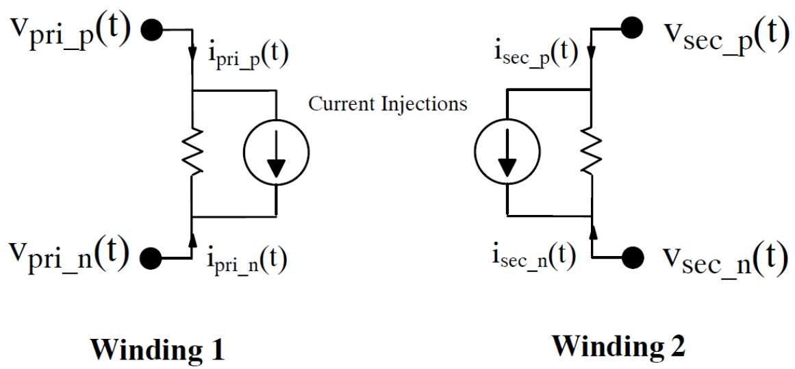 | |
| Figure 8.7: Adjusted Framework for Transformer Model | |
| Equation 8- 10 can then be re- written as Equation 8- 22. | |
| $$ | |
| \begin{array}{r}\left[ \begin{array}{l}i_{pri\_ p}(t)\\ i_{sec\_ p}(t) \end{array} \right] = \left[ \begin{array}{ll}g_{TR_{11}} & g_{TR_{12}}\\ g_{TR_{21}} & g_{TR_{22}} \end{array} \right]\left[ \begin{array}{l}v_{pri\_ p}(t) - v_{pri\_ n}(t)\\ v_{sec\_ p}(t) - v_{sec\_ n}(t) \end{array} \right] + \left[ \begin{array}{l}ih_{pri}(t)\\ ih_{sec}(t) \end{array} \right] \end{array} | |
| $$ | |
| Equation 8- 22 | |
| Knowing that $i_{pri\_ n}(t)$ and $i_{sec\_ n}(t)$ are equal to $- i_{pri\_ p}(t)$ and $- i_{sec\_ p}(t)$ respectively, the generalized matrix equation for our simple transformer can be written as in Equation 8- 23. | |
| $$ | |
| \begin{array}{r}\left[ \begin{array}{l}i_{pri\_ p}(t)\\ i_{sec\_ p}(t)\\ i_{pri\_ n}(t)\\ i_{sec\_ n}(t) \end{array} \right] = \left[ \begin{array}{llll}g_{TR_{11}} & g_{TR_{12}} & -g_{TR_{11}} & -g_{TR_{12}}\\ g_{TR_{21}} & g_{TR_{22}} & -g_{TR_{21}} & -g_{TR_{22}}\\ -g_{TR_{11}} & -g_{TR_{12}} & g_{TR_{11}} & g_{TR_{12}}\\ -g_{TR_{21}} & -g_{TR_{22}} & g_{TR_{21}} & g_{TR_{22}} \end{array} \right]\left[ \begin{array}{l}v_{pri\_ p}(t)\\ v_{sec\_ p}(t)\\ v_{pri\_ n}(t)\\ v_{sec\_ n}(t) \end{array} \right] + \left[ \begin{array}{l}ih_{pri}(t)\\ ih_{sec}(t)\\ -ih_{pri}(t)\\ -ih_{sec}(t) \end{array} \right] \end{array} | |
| $$ | |
| Equation 8- 23 | |
| Where: | |
| $$ | |
| r = \frac{1}{s_{rated}}\left[ \begin{array}{cc}\frac{r_s}{2} v_{rated_1}^2 & 0\\ 0 & \frac{r_s}{2} v_{rated_2}^2 \end{array} \right] | |
| $$ | |
| Equation 8- 24 | |
| $$ | |
| l = \frac{1}{s_{rated}}\left[ \begin{array}{cc}\left(x_m + \frac{x_l}{2} v_{rated_1}^2\right) & x_m v_{rated1}v_{rated2}\\ x_m v_{rated1}v_{rated2} & \left(x_m + \frac{x_l}{2}\right)v_{rated2} \end{array} \right] | |
| $$ | |
| Equation 8- 25 | |
| $$ | |
| g_{TR} = \frac{\Delta t}{2}\left[\frac{[r]\Delta t}{2} +[l]\right]^{-1} = \left[\frac{g_{TR_{11}}}{g_{TR_{21}}}\frac{g_{TR_{12}}}{g_{TR_{22}}}\right] \tag{Equation 8-26} | |
| $$ | |
| $$ | |
| \begin{array}{r}\left[ih_{pri}(t)\right] = [g_{TR}]\left[\left[v_{pri\_ p}(t - \Delta t)\right] - \left[r] - [l]\frac{2}{\Delta t}\right]\left[i_{pri\_ p}(t - \Delta t)\right]\right]\\ ih_{sec}(t)\} = [g_{TR}]\left[\left[v_{sec\_ p}(t - \Delta t)\right] - \left[r] - [l]\frac{2}{\Delta t}\right]\left[i_{sec\_ p}(t - \Delta t)\right]\right] \end{array} | |
| $$ | |
| Equation 8- 27 | |
| Together, Equation 8- 23, Equation 8- 24, Equation 8- 25, Equation 8- 26, and Equation 8- 27 form the equations that will be used to implement the simple transformer example. Details regarding that implementation are given in Section 8.3. | |
| # 8.3 DRAW GRAPHICS AND ADD PARAMETERS | |
| Draw a transformer icon similar to that shown in Figure 8.8. Based on the circuit of Figure 8.5, the component icon for the Simple Transformer should include four (4) power system nodes. The node names to be used are indicated in Figure 8.8. | |
| 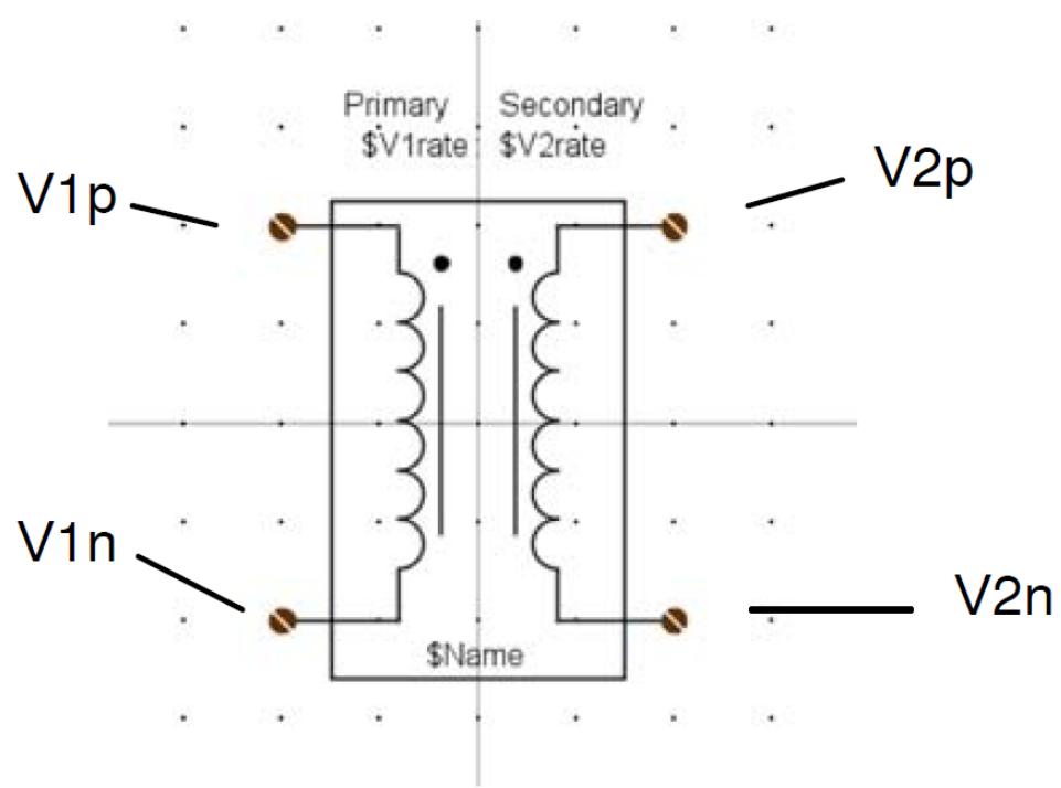 | |
| Figure 8.8: Icon for Simple Transformer Component | |
| Create a new section called 'TRANSFORMER PARAMETERS' and then add an entry for each one of the parameters in Figure 8.9. Default data is shown in the figure. The model includes typical transformer properties such as leakage reactance and series resistance. Being a simple example, no special care has been taken to limit the data entered in these parameters. | |
| # Save the definition file that has just been created as 'SimpleTR.def'. | |
| 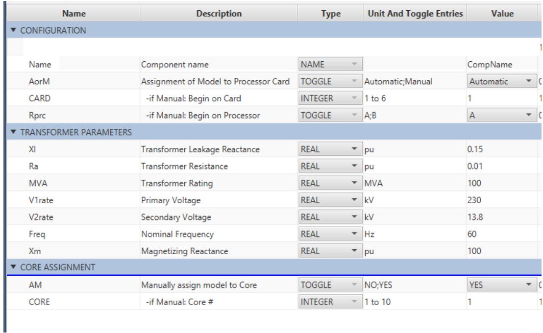 | |
| Figure 8.9: Parameter Data for Simple Transformer Component | |
| # 8.4 ADDING THE MODEL CODE | |
| Select the 'C File Associations' tab.- Add New Association.When a new C File Association is made for the power system component, a menu appears in which the model name must be entered. | |
| Creating the C File Associations for the component automatically generates the following associations: | |
| NODES: V1p, V1n, V2p, V2n (power system nodes) | |
| PARAMETERS: Name[11], XI, Ra, MVA, V1rate, V2rate, Freq and Xm (transformer parameters) | |
| In addition to those listed above, the following additional associations need to be made: | |
| INJECTIONS: A current injection will be made at each of the four power system nodes. To add an injection click the + sign beside the Injections menu. Enter the name for the current injection variable as 'l1p'. After selecting OK the INJECTIONS section is added with the single line representing one current injection association. Select the down arrow icon for the 'l1p' variable and select Node 'V1p' so that the injection is associate with the correct node. The | |
| type would be REAL for all the injections in this case. Add the current injection variables 'l1n', $12p'$ and 'l2n' and then associate them with the appropriate nodes. | |
| 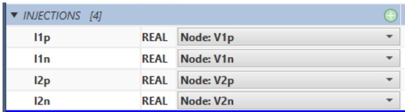 | |
| Figure 8.10: Required Current Injections for the Transformer | |
| Selecting File- $\rightarrow$ Save causes the newly added INJECTIONS variables to be written to the .h file so they can be accessed in the .c file. | |
| # 8.5 BASIC ALGORITHM | |
| 1. When the case is compiled calculate the transformer's contribution to the global G-matrix. The contributions are fixed. | |
| 2. Read four node voltages $V_{1p}(t - 1)$ , $V_{2p}(t - 1)$ , $V_{1n}(t - 1)$ and $V_{2n}(t - 1)$ . | |
| 3. Compute voltages across the primary and secondary windings during the previous time-step, $V_{1}(t - 1)$ and $V_{2}(t - 1)$ . | |
| 4. Use the calculated voltages to calculate the current in each winding at the previous time-step, $l_{1}(t - 1)$ and $l_{2}(t - 1)$ . | |
| 5. Use voltages and currents from the previous time-step to calculate the current injections for the current time-step and pass them to the network solution. | |
| 6. Let the network solution complete the calculation of something similar to Equation 8-23 and then return to step 2 at the next time-step. | |
| The contributions of the Simple Transformer to the global conductance matrix are fixed and do not vary with time. Because of this, these contributions only need to be calculated once when the simulation is being compiled. This will save both computation and communication time compared situations when the model's conductance contributions must be calculated every time step. | |
| Setting up the contributions is fairly straight forward but requires that initialization code be placed in the RAM_PASSs1 section instead of the RAM section. It also requires that calls be made to some special functions which are listed in the code below. | |
| Click "Edit C File" button to start editing the C code. | |
| CBuilder Tutorial: Simple Transformer | |
| // Simple Transformer Tutorial Example// E RTDS Technologies, Inc.// Written by Gregory Jackson// August 22nd, 2013 | |
| include "simpleTR01. h" | |
| // Declare some variable that will be// used in the RAM_PASS1 and CODE sections | |
| # STATIC: | |
| double v1_old, v2_old; double i1_old, i2_old; double i11, i11_old, i12, i12_old; double dt; double R11, R12, R21, R22; double L11, L12, L21, L22; double Gtr11, Gtr12, Gtr21, Gtr22; double A, B, C, D; double M11, M21; | |
| # RAM: | |
| RAM_PASS1: //read the simulation time- stepdt = getTime- step(); | |
| //Determine which row and column in the G- matrix is //associated with each node. The first statement below, //for example, associates row and column 1 of the G //matrix to node "V1p". The 'g_mat_nods[]' array is //reserved and must be used. g_mat_nods[0] = getNodeNum(comp,"V1p"); g_mat_nods[1] = getNodeNum(comp,"V2p"); g_mat_nods[2] = getNodeNum(comp,"V1n"); g_mat_nods[3] = getNodeNum(comp,"V2n"); | |
| # //Calculate Elements of the R and L matrices [Eq. 24] | |
| $\mathsf{R11} = \mathsf{Ra}^{*}0.5^{*}\mathsf{V1rate}^{*}\mathsf{V1rate} / \mathsf{MVA};$ $\mathsf{R12} = 0;$ $\mathsf{R22} = \mathsf{Ra}^{*}0.5^{*}\mathsf{V2rate}^{*}\mathsf{V2rate} / \mathsf{MVA};$ $\mathsf{R21} = 0;$ | |
| $\mathsf{L11} = (\mathsf{Xm} + \mathsf{Xl}^{*}0.5)^{*}\mathsf{V1rate}^{*}\mathsf{V1rate} / \mathsf{MVA};$ $\mathsf{L12} = \mathsf{Xm}^{*}\mathsf{V1rate}^{*}\mathsf{V2rate} / \mathsf{MVA};$ $\mathsf{L21} = \mathsf{Xm}^{*}\mathsf{V1rate}^{*}\mathsf{V2rate} / \mathsf{MVA};$ $\mathsf{L22} = (\mathsf{Xm} + \mathsf{Xl}^{*}0.5)^{*}\mathsf{V2rate}^{*}\mathsf{V2rate} / \mathsf{MVA};$ | |
| // Calculate the elements of the transformer's G- matrix// The inversion of a 4x4 matrix is completed. [Eq. 25]A = R11*dt/2 + L11;B = R12*dt/2 + L12;C = R21*dt/2 + L21;D = R22*dt/2 + L22; | |
| Gtr11 = dt/(2*(A*D- B*C)) * D; Gtr12 = dt/(2*(A*D- B*C)) * - B; Gtr21 = dt/(2*(A*D- B*C)) * - C; Gtr22 = dt/(2*(A*D- B*C)) * A; | |
| //Setup the G- matrix for the transformer. [Eq. 23] //g_mat_over[][] is a reserved array that must be used. //The conductance matrix is fixed so it only needs to be //calculated once here when the case is compiled. g_mat_over[0][0] = Gtr11; g_mat_over[0][1] = Gtr12; g_mat_over[0][2] = - Gtr11; g_mat_over[0][3] = - Gtr12; | |
| g_mat_over[1][0] = Gtr21; g_mat_over[1][1] = Gtr22; g_mat_over[1][2] = - Gtr21; g_mat_over[1][3] = - Gtr22; | |
| g_mat_over[2][0] = - Gtr11; g_mat_over[2][1] = - Gtr12; g_mat_over[2][2] = Gtr11; g_mat_over[2][3] = Gtr12; | |
| g_mat_over[3][0] = - Gtr21; g_mat_over[3][1] = - Gtr22; g_mat_over[3][2] = Gtr21; g_mat_over[3][3] = Gtr22; | |
| //Pass the component's G- matrix contributions to the main//network solution. The function's argument is the//dimension of the component's G- matrix.setupGMatrix(4); | |
| CODE: | |
| # BEGIN_TO: | |
| //Calculate the voltage across each of the transformer's// windings at the previous time- step.v1_old = V1p- V1n;v2_old = V2p- V2n; | |
| //Calculate the current flowing in//each winding at the previous time- step.i1_old = Gtr11*v1_old + Gtr12*v2_old + IH1_old;i2_old = Gtr21*v1_old + Gtr22*v2_old + IH2_old; | |
| //Calculate the transformer's history currents [Eq. 26]M11=v1_old- (R11- L11*2/dt)*i1_old- (R12- L12*2/dt)*i2_old;M21=v2_old- (R21- L21*2/dt)*i1_old- (R22- L22*2/dt)*i2_old; | |
| IH1 = Gtr11*M11 + Gtr12*M21;IH2 = Gtr21*M11 + Gtr22*M21; | |
| //Keep track of old history terms IH1_old = IH1;IH2_old = IH2;//Current injections: a - ve value implies the current//flowing into a node;a +ve value implies the current is | |
| # //flowing out of a node | |
| $$ | |
| \begin{array}{l}{11p = \mathsf{IH1};}\\ {}\\ {11n = \mathsf{-IH1};}\\ {}\\ {12p = \mathsf{IH2};}\\ {}\\ {12n = \mathsf{-IH2};} \end{array} | |
| $$ | |
| TO_T2: | |
| After adding the code, try to compile your model. If successful, add the Simple Transformer into DRAFT and build a simple test circuit such as the one shown in Figure 8.11. For the sake of stability, it is important to have a reference to ground on each winding of the transformer. | |
| 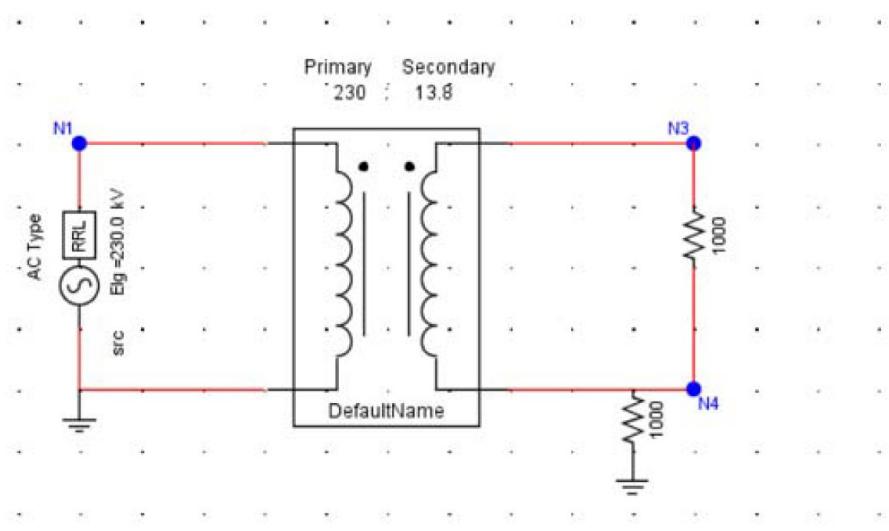 | |
| Figure 8.11: Simple DRAFT Case used to Test Simple Transformer Model | |
| After compiling and running the DRAFT case you should be able to observe the correct voltage ratio between the primary and secondary sides of the transformer. You should also be able to observe the load voltage drop as the secondary side load impedance is reduced. This will be due to the voltage drop across the transformer's leakage reactance and winding resistance. | |
| # 8.6 REFERENCES | |
| [1] Electro- Magnetic Transients Program (EMTP) Theory Book. Hermann W. Dommel. 1987. | |
| # 9 | |
| # MULTIPLIER WITH COMPLEX NUMBERS AS INPUTS | |
| # 9.1 INTRODUCTION | |
| The component can multiply 2 or 3 complex number inputs. The operation mode can be set to either polar or rectangular form. | |
| # 9.2 CREATE THE REQUIRED PARAMETERS | |
| The goal is to draw a component icon that looks similar to Figure 9.1. | |
| 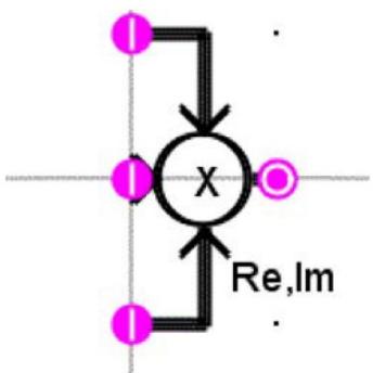 | |
| Figure 9.1: Multiplier with Complex Numbers as Inputs Component Icon | |
| Ensure to create conditional graphics for the third input line i.e. if (numInputs==1) condition is selected and draw the third input line. You can even add text (under condition, Mode==1) to indicate the operational mode. Refer to chapter 1 for detailed graphics drawing instructions. | |
| Add the following parameters. | |
| # Parameter #1 | |
| Parameter #1Name: numInputsDescription: Number Of InputsType: TOGGLEUnit/Toggle Entries: Two; Three | |
| # Parameter #2 | |
| Parameter #2Name: ModeDescription: Operation modeType: TOGGLE Unit/Toggle Entries: Re,IM; |X|,∠X | |
| # 9.3 ADD THE IO POINTS | |
| In this example some of the IO points are conditional. Start by making the conditions for the IO points. | |
| Select the 'IO Points' tab.- Create a condition so the IO Points table appears similar to Figure 9.2. | |
| 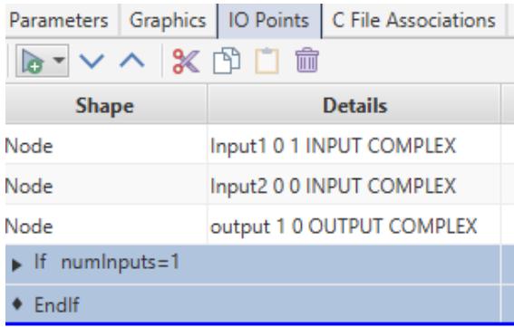 | |
| Figure 9.2: Condition Created in IO Points Tab | |
| Select condition 'IO Points' (highlighted in Figure 9.2). Using the IO point tool, place a new IO point where the Input1 connection should be. | |
| You will be prompted for IO point information. Enter the information below. | |
| # IO point Input1 | |
| Name: Input1 | |
| conn: SIGNAL INPUT | |
| var: COMPLEX | |
| Type: EITHER | |
| Condition: Mode $= = 0$ | |
| The COMPLEX IO point supports Re, Im or |X|, ∠X or both types of inputs. The Type value is used to set the particular type of input. If Either is selected for Type, then a | |
| condition must be specified based on which input type will be selected. If the condition evaluates to True, then a Re, Im type input is expected. In this case we will use Mode $= = 0$ as the condition. For example, if the selected mode was 'Re, Im', the condition (Mode $= = 0$ ) evaluates to true and real and imaginary type inputs are expected. Input1[0] will hold the Real part and Input1[1] will hold the Imaginary part of the complex number. If the selected Mode is $|X|$ , $\angle X$ , the condition evaluates to false and magnitude and angle inputs are expected. Input1[0] will hold the magnitude part and Input1[1] will hold the angle part of the complex number. | |
| - Repeat the above process for IO point Input2 and output.- Next add Input3. Before adding Input3 IO point, select the condition 'If numInputs $= = 1$ '. | |
| # 9.4 ADDING THE MODEL CODE | |
| - Select the 'C File Associations' tab.- Select the Add New Association.- Enter a model name such as 'cpxMul'.- The associations should appear similar to those in Figure 9.3. | |
| 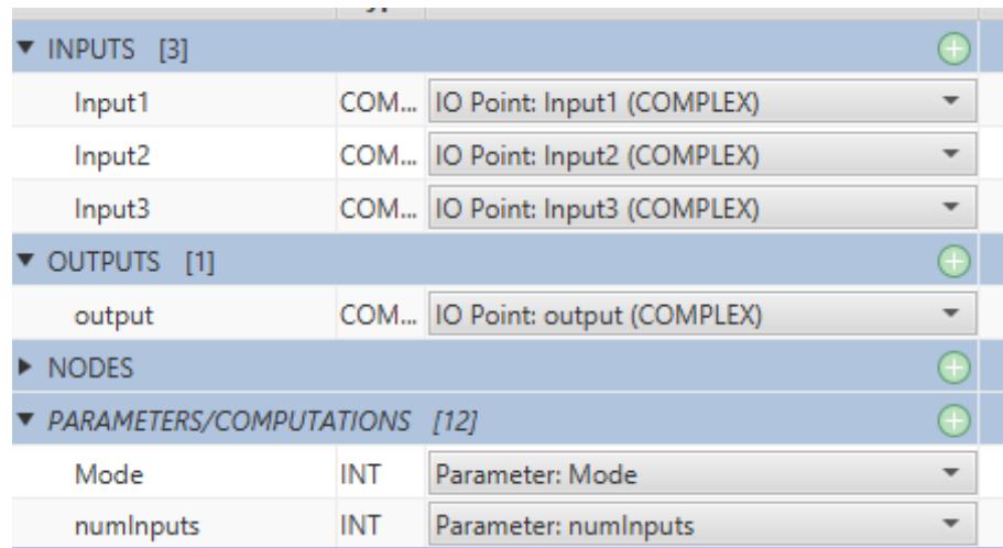 | |
| Figure 9.3: Associations | |
| - Edit the .c file. | |
| - After writing the 'c' code, select the compile button to compile the code. If the compile is successful, the component is ready to be included in a Draft circuit. | |
| - Ensure that the component builder icon is saved. | |
| # 9.5 SAMPLE 'C' CODE FOR THE MULTIPLE INPUT MULTIPLIER WITH COMPLEX NUMBER INPUTS STATIC: | |
| double RL,IM; | |
| RAM FUNCTIONS: | |
| RAM: | |
| CODE: | |
| if(Mode $= = 0$ {RL=(Input1[0]\*Input2[0]- Input1[1]\*Input2[1]);IM=(Input1[0]\*Input2[1] $^+$ Input1[1]\*Input2[0]);if(numInputs $= = 1$ {output[0]=RL\*Input3[0]- IM\*Input3[1];output[1]=RL\*Input3[1] $^+$ IM\*Input3[0];}else{output[0]=RL;output[1]=IM;}}else{if(numInputs $= = 1$ | |
| # Builder Tutorial: Multiplier with Complex Numbers as Inputs | |
| {output[0]=Input1[0] * Input2[0] * Input3[0];output[1]=Input1[1] + Input2[1] + Input3[1];}else{output[0]=Input1[0] * Input2[0];output[1]=Input1[1] + Input2[1];} |
This file contains hidden or bidirectional Unicode text that may be interpreted or compiled differently than what appears below. To review, open the file in an editor that reveals hidden Unicode characters.
Learn more about bidirectional Unicode characters
| # CBUILDER User's Manual | |
| APRIL 2012 | |
|  | |
| # User Defined Component Models in C | |
|  | |
| # TABLE OF CONTENTS | |
| 1 Introduction to CBuilder 1.1 | |
| 1.1 Steps in Building A New RTDS Component 1.2 | |
| 2 Drawing the Component 2.1 | |
| 2.1 Macros 2.7 2.2 Adding Input/Output Points & Nodes 2.10 2.3 Selecting & Manipulation of Shapes 2.11 2.4 Using the Grid Properties 2.16 2.5 The Graphics Tab 2.24 2.6 Mirror and Rotate Options 2.25 2.7 Adding Logic Blocks to the Component Icon 2.27 2.8 Single Line Diagram (SLD) 2.32 | |
| 3 Component Parameters 3.1 | |
| 3.1 Adding a New Parameter to a Section 3.2 3.2 Editing an Existing Parameter 3.7 3.3 Adding a New Section 3.8 3.4 Moving or Copying Parameters into a Section 3.9 | |
| 4 Source Code for the Component Model 4.1 | |
| 4.1 Creating the C File Associations 4.3 4.2 Illustrative Example 4.5 4.3 Data Preparation Portion of the C Code 4.6 4.4 RTDS Executable Portion of the C Code 4.8 4.5 Limitation on the use of Output Variables 4.9 4.6 Compiling and Testing the Component Model 4.10 4.7 Modifying an Existing Component 4.11 4.8 Adding a Function to the C Code 4.17 4.9 C Code for a Power System Component Model 4.18 | |
| # 4.10 Power System Component (Illustrative Example) 4.20 | |
| 5 Computations Tab 5.1 5.1 Checks Tab 5.3 5.2 Other Tab 5.4 | |
| Appendix A: Available Parameter Types A.1 Appendix B: Functions Available in the Data Prep. Code A.2 Appendix C: Functions Available in the RTDS Exec. Code A.3 Appendix D: Operators Available in the RTDS Exec. Code A.9 Appendix E: Generic Controls available in Cbuilder A.10 Appendix F: Memory Allocation A.23 Appendix G: Complex Numbers A.25 Appendix H: Halt() and reportError_RW() A.26 Appendix I: Maintaining DLL files A.27 Appendix J: Calling functions with the same name in different CBuilder models A.28 | |
| RSCAD's CBuilder software module provides a mechanism for RTDS users to develop their own component models. Both power system and control system type components may be developed using CBuilder. Prior to the introduction of CBuilder the UDC(User Defined Component) software was available to users for the development of custom models in RTDS. The CBuilder software builds on the capabilities that were included in the UDC and provides a more user friendly environment in which to build the component models for the GPC/PB5 Processor Cards available with the RTDS. | |
| CBuilder includes an interface for drawing the component's icon including its appearance in 3 Phase and single line diagram modes in RSCAD/Draft. It also provides the structure to define the parameters which must be entered by the user for the new model, as well as, a mechanism to provide input and output signals to/from the component. A compiler is included which converts the user written C code for the model into executable code which is integrated into the RTDS software library. Upon successful compilation, the user's new model may be included within simulation cases prepared in RSCAD/Draft just as any other component from the RTDS libraries. The user's component model may be shared with other RTDS users. Only the compiled code and component icon file needs to be available for other users to include the new component into their simulation cases. | |
| The CBuilder software is available in RSCAD Version 2.00 and above. To start the CBuilder software left click the CBuilder icon from RSCAD/FileManager. | |
|  | |
| To create a new component using CBuilder, select the New File radio button and select Ok from the Welcome menu that appears after starting CBuilder. Select whether the new component will be a control system component or a power system component. Note that only power system components may directly connect to power system nodes. Control type components may obtain input from other control type components or by measuring power system signals such as node voltages or branch currents. | |
| The steps required to generate a new component using CBuilder are as follows - | |
| i) Draw the component using shapes from the shapes menu ii) Allocate input and output points iii) Define the component's parameters (parameters are entered into the component's menus by the user in RSCAD/Draft). iv) Write the C Code for the data preparation portion v) Write the C Code for the algorithm that runs on the RTDS vi) Compile the new model from within CBuilder vii) Load the new component model in RSCAD/Draft and test it in a simulation case. | |
| The following chapters of this manual provide information regarding the above steps. The user is also directed to the CBuilder Tutorial Manual where more substantial component models are documented. | |
| The graphic representation of the component is assembled from basic shapes which are placed in the drawing area of the CBuilder window. The drawing area is visible only when the Design tab located near the top left side of the CBuilder screen is selected. The graphic created by the user under CBuilder will be seen as the component in RSCAD/Draft. It is possible to place logic blocks around the various shapes comprising the component so that the component's appearance can change depending upon parameters selected by the user in RSCAD/Draft. | |
| For power system components, the user must create two component images. One is displayed when the 3 Phase view mode is selected in RSCAD/Draft and the other when the single phase view mode is selected. | |
| # COORDINATE SYSTEM | |
| The drawing area by default includes a grid system with 32 pixel spacing. Light grey lines are used to define the coordinate axes with the 0,0 point located where the two grey lines cross. The 0,0 point can be displayed at the center of the drawing area by left clicking the go to 0,0 button located near the top left hand corner of the CBuilder window. | |
| center the drawing area around the 0,0 point | |
| The 0,0 point in the drawing area is used as the center point for the component being constructed. If the component is drawn such that it is symmetrical around the 0,0 coordinate, then the rotate and mirror commands in RSCAD/Draft will result in the component moving about its center. | |
| Wire components in RSCAD/Draft may only terminate on 32 pixel grid points. As such, any input and output connection points on the component must terminate on a 32 pixel grid point. | |
| See the section "Using the Grid Properties" below for more information regarding the grid. | |
| # BASIC SHAPES | |
| In order to place basic shapes onto the drawing area, ensure that the Design tab is selected. The shapes toolbar is located to the right of the drawing area and includes the basic shapes as shown below. | |
| To place a particular shape in the drawing area left click on the desired shape and move the cursor (the cursor changes from an arrow to cross hairs) onto the drawing area. Click and hold the left mouse button to start drawing the selected shape. Move the cursor while holding the left mouse button to stretch the shape to its desired size. Release the left mouse button to complete drawing of the component. The cursor changes back to an arrow. See the section of this manual entitled "Using the GRID Properties" regarding alignment of the shape to the drawing area's grid. | |
|  | |
|  | |
| To draw multiple instances of the same shape, double left click the desired shape button. The button remains highlighted. Draw the shape as described above. Once completed, however, the cursor remains as a crosshair and another of the same shape can be drawn. When complete left click the highlighted component or another shape button. | |
| # ARC | |
| To draw an arc, select the draw arc button and left click when the cross hair cursor is over the desired center point of the arc. The arc shape requires that the user specify the arc's radius and angle extent in a pop up that appears after left clicking to place the arc shape. The diagram below gives some examples of arc's and their coordinate specifications. | |
|  | |
|  | |
|  | |
|  | |
|  | |
|  | |
| # TEXT | |
| To place a single line of text on the drawing area, left click the text shape in the drawing menu and move the cursor to the desired position on the drawing area. The text is centered around the position selected for the text. A popup menu appears in which the x,y coordinate of the center point may be specified (the initial x,y coordinates in the popup are based on the position of the cursor when the text was dropped). Three types of text components are available. | |
| LABEL: A line of text which is displayed as typed (including spaces). Labels may be placed within logic blocks in the graphics section so that they will appear in the RSCAD/Draft component icon only if the associated logic is true. | |
| VAR: Displays the value of a parameter. For example, the component's name is often provided with the "Name" parameter. To display the component's name in RSCAD/Draft enter the box labelled text and select the type as var. The text "\(\) \text{Name}\)" appears in the drawing area to indicate that the text is to be replaced by a parameter value. | |
| BOTH: Displays both the parameter name and value in the RSCAD/Draft component. For example, to display the processor type to which the component is assigned enter "prtyp" in the box labelled text and specify the type as both. The text "prtyp=\(\) \text{prtyp}\)" appears in the drawing area. In RSCAD/Draft the text appears as "prtyp=GPC/PB5" if the processor type is selected as GPC/PB5 by the user. | |
|  | |
| # INSERT AN IMAGE FILE | |
| INSERT AN IMAGE FILEImages can be included into the user component by left clicking on the add image icon in Cbuilder. The image to be included must be placed in the same directory as the component. By default new Cbuilder components are located in the RTDS_USER\ULIB directory. This feature only supports images with a .JPG and .GIF extension. | |
|  | |
| Macros are shapes comprised of a number of basic drawing elements. The list of available macros may be seen by left clicking the button labelled "Macro▶" and selecting one of the available sub- menus and then the desired component. | |
| It should be noted that macros are not the same as a group of shapes (although a macro may be converted to a group of shapes, see below). Drawing instructions for the macro are contained in a file (filename.g). | |
| The user may choose to add one or more macros to the drawing component menu located just under the button labelled " Frequent". Left click the frequent button and select the macros to be added to the drawing component menu by left clicking in the small box located to the left of the component. Click once to add the macro to the menu (a check mark appears), click again to remove the macro from the menu. | |
|  | |
| When a macro is placed onto the drawing area it is treated as a single component by default. It is possible to break the macro component into its constituent parts by selecting the component (left click when the cursor is over the macro) and then left clicking the box labelled "Break Down". The macro component is replaced by its basic shapes (lines, arcs, text etc.). Another option is to select "Make Group" when the macro is selected. In this case the macro is again converted to its constituent shapes, but these shapes are assembled as a group. | |
| Macro components may not be rotated or flipped. To change the appearance of a macro first change it to individual shapes by using either the "Break Down" or "Make Group" options. | |
|  | |
| When a component which includes macros is saved, the reference to the macro is saved as part of the component. If the file containing the macro is changed, those changes will be seen in all components which reference that macro. Using the "Break Down" or "Make Group" removes the reference to the macro and the information associated with the individual shapes is saved as part of the component. | |
| A user can save grouped individual drawing elements as a macro. See section 2.3 on grouping individual drawing elements. Left clicking on the "Save as Macro" button saves the grouped ele- | |
| ments as a macro in the RTDS_USER\ULIB directory with a g extension. The macro will then be added to list of available macros and may be seen by left clicking the button labelled "Macro▶" and selecting the macro from the available sub- menus. | |
|  | |
|  | |
| Input and Output points are those points associated with a component to which wires are connected in RSCAD/Draft in order to interconnect the new component with other components. Input and Output points refer to signals associated with control blocks or monitored signals. Input and Output points may be specified as either real or integer and are distinct from Power System Nodes. Input and Output points may be included with both control and power system type components while Power System Nodes may only be associated with power system type components. Adding a Node to a power system component defines a power system Node in the circuit into which the component is placed. Input/Output points and Power System Nodes may only be placed on 32 pixel grid points. | |
| Left clicking the create point button facilitates the placing of an Input or Output point or a Power System Node (power system type component only) in the drawing area. The type of component is specified in the menu that appears once the point has been placed on the drawing area. | |
|  | |
| The name assigned to the input or output point is used as the variable name in the C code that must be written for the new component. The normal rules for variable names apply (no spaces, may not start with a number, may not include special characters, maxi | |
| mum name length is 20. ). Input point variable names must appear on the right side of an expression and output point variable names on the left side. For example - | |
| MYOUTVAR= 2.0\*VAR1; VAR2= MYINPVAR \* 5.0; | |
| # 2.3 SELECTING & MANIPULATING SHAPES | |
| Once the basic shapes comprising the compound have been drawn it is possible to manipulate the shapes using various options. To manipulate a shape it must be selected. A shape may be selected by moving the cursor over the shape's outline (the shape highlights to indicate it will be selected) and left clicking. The shape remains highlighted after the cursor is moved away. | |
| Multiple shapes may be selected by holding the shift key down when left clicking. It is also possible to select multiple shapes by placing the cursor over the drawing area (not over a component) and while the left mouse button is pressed dragging the cursor over the components that are to be selected. Any components fully encompassed by the light grey selection box become selected. Not all shape manipulations are possible when multiple shapes are selected. | |
| Selecting a shape which is a group of multiple shapes allows only the ungroup shape option. | |
| The following options are available to change the appearance of selected components. | |
| OUTLINE COLOUR: Left click the $\triangledown$ icon next to the Outline box to select the desired outline colour. This option is available when multiple shapes are selected. Any parameters defined as type COLOR will appear in the OUTLINE COLOR pulldown menu. Choosing the parameter name rather than a fixed color permits the user to change the shapes' color from RSCAD/Draft. | |
| OUTLINE THICKNESS: Enter the desired outline thickness in the text box to the right of the outline colour selection box. Outline thickness is in pixels with a minimum value of 1. This option is available when multiple shapes are selected. A parameter value rather than a constant may be entered by prefixing the parameter name with a $\Phi$ character. For example, if the parameter LW has been defined as type INTEGER then $\Phi \mathrm{LW}$ may be entered in the outline width box. If the user changes the value of LW in RSCAD/ Draft then all shapes using LW for their width will change appearance. | |
| OUTLINE STYLE: Left click the $\triangledown$ icon located to the right of the line style indicator box and select the desired line style (Solid or Dashed). This option is available when multiple shapes are selected. | |
| FILL: This option is under development. | |
| Shape appearance manipulation menu | |
|  | |
| The following options are available to manipulate the position, size and orientation of selected components. | |
| MOVE: Placing the cursor over the outline of an already selected image causes the cursor to change to a compass style. Left clicking and dragging when the cursor is displayed as a compass style causes the selected shape to be moved. | |
| It is also possible to move the shape by entering the x,y coordinates into the x:, y: boxes which appear when the shape is selected. | |
|  | |
| MOVE ONE GRID SPACE: Selected components can be moved one grid point by left clicking one of the grid point move buttons as shown below. | |
|  | |
| SIZE: A selected shape includes a number of stretch points (indicated as small boxes on the shape's outline). Moving the cursor over one of these stretch points results in the cursor changing to a diagonal arrow. Left clicking and dragging stretches the shape. | |
|  | |
| It is also possible to resize a shape by entering the end point coordinates into the x,y boxes as shown above. | |
| ROTATE & FLIP: Selected components may be rotated by 90 deg., flipped horizontally, vertically or diagonally by left clicking the buttons as shown below. | |
|  | |
| GROUP & UNGROUP: A number of shapes can be arranged into a group. Once arranged as a group any manipulation applies to all shapes comprising the group. The ungroup command returns all of the individual shapes. Both Group and Ungroup commands follow a hierarchy. Thus, applying Group to two sets of shapes which are already groups causes a new group to be formed containing the two groups. Using the ungroup command causes the initial two groups to be returned. | |
| Grouped shapes are only maintained for the current RSCAD/ CBuilder session. Saving the component, closing and then re- | |
| opening CBuilder removes all group information. | |
| Select the shapes that are to be grouped and left click the group button. The selected shapes become a single shape. Select the grouped shape and left click ungroup to return the initial shapes as individual shapes. | |
|  | |
| MOVE TO FRONT OR BACK: Shapes may be placed in front of or behind other shapes. Buttons exist to move a shape to the front, to the back, move a shape one level up or one level down. A new shape is always drawn on the top level over existing shapes. Selecting the new shape and then left clicking move backward causes the new shape to be drawn one level down (ie. behind) from the previously drawn shape. | |
|  | |
| A grid is provided in the drawing area to help align the various shapes comprising the component. Default spacing on the grid is 32 pixels for both the x and y axes. A light grey horizontal and vertical line are provided on the grid to show the coordinate axes. The 0,0 point on the drawing grid is used as the center point for the component being drawn. The 0,0 point of the component is used for the axis of rotation when the rotate command is selected for the component in RSCAD/Draft. The effect of the rotate command when the component is not centered around the 0,0 point is shown below. The 0,0 point of the drawing area can be brought to the center of the display by left clicking the go to (0,0) button located on the main toolbar. | |
| center the drawing area around the 0,0 point | |
|  | |
| component is not centered around the 0,0 point | |
|  | |
| component is centered around the 0,0 point | |
| Application of ROTATE Command in RSCAD/Draft | |
| Power system nodes, as well as, input and output points may only be located on the 32 pixel grid dots. Other drawing elements may be placed arbitrarily on the drawing area. To assist in placing the shape elements the following grid related options are available from the grid selection toolbar located just above the drawing area | |
|  | |
| # ZOOM GRID 170 | |
| Use the slider or enter a value in the $\%$ box located to the right of the slider to zoom in (or out) the drawing area. The zoom range is limited to $50 - 800\%$ . The center point in the drawing area is used as the point around which to zoom. | |
| To zoom in (or out) on a particular point on the drawing area the magnifying $^{\ast} + ^{\ast}$ or $- ^{,,}$ buttons may be used. Left clicking either of these buttons changes the cursor to the magnify icon. Left clicking with the magnify cursor zooms in by $+ / - 40\%$ on the selected point on the drawing canvas. Holding the Ctrl key when left clicking with the magnify icon displayed causes the magnification to change sign. | |
| # DISABLE SNAP FEATURE | |
| Left clicking the disable snap feature permits shapes to be placed in arbitrary locations relative to the 32 pixel grid on the drawing area. Note that only one of the Snap options may be selected at one time (Disable Snap, Snap to Shape, Snap to Grid (Relative) and Snap to Grid (Absolute) operate as radio buttons). | |
| Power system node and input/output points are always placed on 32 pixel grid locations, irrespective of the selected snap option. | |
| # SNAP TO SHAPE | |
| Left clicking the snap to shape button causes new shapes to be drawn such that their end points or corners are connected. The point to which the new shape will snap is indicated by a small red circle which appears when the drawing cursor is moved near an existing component on the drawing area. | |
| Both the start and end points of the new shape component will snap to an existing shape's endpoint when the cursor is brought near that component. | |
|  | |
| start point indicated by red circle when the cursor is moved near an existing shape's end point end point indicated by red circle once drawing of the shape has begun and the cursor is moved near an existing shape's end point. | |
| # SNAP TO GRID (RELATIVE) | |
| Left clicking the snap to grid (relative) button is only relevant when moving shapes (either moving an existing shape or moving a shape which was copied). Components being moved will snap to a grid location with the same relative offset as the shape's original position. If a shape was placed while the disable snap feature was selected it could be placed any number of pixels away from a grid point. When moving the shape it can be placed only the same number of pixels away from another grid point. | |
|  | |
| original line drawn with disable snap feature was selected and placed such that its end point was offset from the nearest grid point. | |
| when the line is moved, its new location is relative to a grid point with the same x and y offset as the original position | |
| # Snap to Shape Feature Enabled | |
| Using the move buttons from the main toolbar when the snap to | |
| grid (relative) button is selected permits the selected component to be moved by one grid position. The component is moved such that the relative position to a grid point remains the same. | |
|  | |
| # SNAP TO GRID (ABSOLUTE) | |
| Left clicking the snap to grid (absolute) button causes shapes to be drawn starting and ending on grid points. A red circle appears around the grid point to which the shape will snap. The grid point | |
| to which the shape snaps includes the non 32 pixel boundary grid points which appear if the grid point density is increased. | |
|  | |
| start point indicated by red circle when the cursor is moved near a grid point end point indicated by red circle once drawing of the shape has begun and the cursor is moved near another grid point | |
| Snap to Grid Feature Enabled | |
| # GRID POINT DENSITY SETTING | |
| The number of grid points between the default 32 pixel grid array may be set from the grid point density pull down. The following options are available – | |
|  | |
| Intermediate grid points may be used with any of the snap to grid options discussed above. Nodes and input/output points will always snap to the 32 pixel grid points (shown in black). | |
|  | |
| 32/2 Grid Density | |
| Left clicking on the tab labelled Graphics for control type components or 3Phase/SLD Graphics for power system type components shows a list of the shapes that have been placed on the drawing area. The shapes are drawn in the order in which they appear in the list. To move one component up or down in the list, left click the up or down arrow located on the right side of the line for the shape to be moved up or down one position. If the shape is selected by left clicking its outline in the drawing area, the page up, page down, home and end keys may be used to move the shapes entry in the graphics area up, down, to the top and to the bottom. | |
| Left clicking under the shape column on a line in the Graphics section causes the line to become selected (the line turns red) and the corresponding shape in the drawing area is automatically selected. Left click again to de- select the shape. | |
| A shape may be deleted by left clicking the trash icon or edited by clicking the pencil icon. | |
| Logic blocks may be inserted into the list of shapes (see the next section) so that the shapes are drawn only if a parameter meets a particular condition. | |
|  | |
| Mirror and Rotate options are available from a pulldown associated with selected components in RSCAD/Draft. The Mirror command causes the component to appear as if it were reflected horizontally. Rotate causes the component to rotate clockwise 90 degrees. It is possible to associate NOMIRROR and NOROTATE commands with a shape so that the shape remains in a fixed position even if mirror or rotate commands are issued in RSCAD/ Draft. One of the applications for the NOMIRROR and NOROTATE commands is to keep a label in a fixed position even though the component orientation may be changed by the user. | |
| The nomirror and norotate options can be added to a component by selecting the appropriate check box on the command line for the shape. The command line for the shape can be seen under the Graphics tab and the shape's command line is highlighted when the shape is selected on the drawing area. | |
| # CBuilder: Drawing the Component | |
|  | |
| It is possible to have user selected parameter values change the appearance of the component in RSCAD/Draft. To accomplish this logic blocks may be placed around shape drawing commands. Each shape that is placed in the drawing area adds a new instruction into the list visible when the Graphics tab is selected on the right side of the CBuilder window. Selecting a shape in the drawing area causes the corresponding drawing command to be highlighted. | |
|  | |
| # ADDING A NEW LOGIC BLOCK | |
| To add a new logic block click the add condition button located near the top left of the Graphics command area and select the desired condition from the pull down menu. For example, if the lower arrow (right arrow macro and line shapes in the above Figure) was to be shown only if the parameter input2 was set to "Yes" then the If option should be selected from the pulldown as shown below. | |
| # CBuilder: Drawing the Component | |
|  | |
| The parameter input2 referred to in the Add Condition box shown above should be defined as a toggle type parameter whose selections are specified as 'No' or 'Yes', in that order. If the user selects No then parameter input2 is assigned the value 0 otherwise if Yes is selected then input2 is assigned 1. (See TOGGLE in the Parameters Section for details). | |
| Once the logic condition has been added, the following two lines appear in the shape command area - | |
| If (input2 > 0) EndIf | |
| Any new shapes placed on the drawing area while the If - EndIf commands are highlighted will be placed inside the selected logic and will only be visible if the logic is true. | |
| Existing shape commands can be moved into the logic block by first selecting the shapes and then left clicking the move/copy selected shapes button. Click the Copy or Move radio button to select the desired action. Select the desired logic block into which to Copy or Move the selected shapes by left clicking on the If- EndIf block in the menu that appears followed by Ok. | |
| # CBuilder: Drawing the Component | |
|  | |
| Shapes may be selected either by left clicking when the cursor is over the shape in the drawing area or alternatively by left clicking the shape's command from the command list under the Graphics Tab. Left clicking an already selected shape or command causes the shape to be no longer selected. | |
| # AVAILABLE LOGIC BLOCKS | |
| The following logic blocks may be added to the command list by selecting selecting the appropriate menu item from the Add Condition pull down menu. | |
| If: The basic If- EndIf block | |
| If (condition) EndIf | |
| Else: An Else block may be added to an existing If- EndIf block by first selecting the If- EndIf block and then adding the Else. The resulting logic block appears as - | |
| If (condition) Else EndIf | |
| ElseIf: An ElseIf block may be added to an existing If- EndIf or If- Else- EndIf block by first selecting the logic block and then adding the ElseIf and filling in the desired logic. The resulting logic block appears as - | |
| If (condition) ElseIf (condition) Else EndIf | |
| IfNot: commands within the IfNot logic blocks are executed only if the condition is not true. The condition specifies a parameter followed by a | |
| IfNot (condition) EndIf | |
| The basic structure of the condition within the logic blocks described above is - | |
| parameter logic parameter parameter logic value | |
| Some examples include - parameter1 == parameter2 | |
| # parameter $>0$ | |
| Valid logic statements include - | |
| $= =$ equals $! =$ not equal $>$ greater than $> =$ greater than or equal $<$ less than $< =$ less than or equal | |
| Power system components may be viewed in 3 Phase or Single Line Diagram (SLD) mode within RSCAD/Draft. How the component appears in either mode is determined by the drawing commands under the 3- Phase and SLD drawing modes available under the Graphics tab in CBuilder. It is recommended that the 3- Phase drawing be completed first. The shapes and associated drawing logic for the 3 Phase view can then be copied to the SLD view and modified accordingly. | |
| By default, the SLD drawing mode is not enabled for the component. If no SLD drawing instructions are included with the component, the component's appearance does not change when the view mode is changed from 3 Phase to SLD in RSCAD/Draft. The SLD drawing mode can be enabled by left clicking the button labelled "add SLD Graphics" when the Graphics tab is selected. The SLD radio button becomes active once the SLD Graphics has been enabled and the "3- Phase/SLD" button changes to "3- Phase". Shapes placed onto the drawing area when the SLD radio button is selected only appear in RSCAD/Draft when the SLD mode is selected. | |
|  | |
| When the SLD Graphics mode is first enabled a popup menu appears asking whether the 3- Phase graphic shapes and logic should be copied to the SLD mode. In most cases the SLD version of the component is closely related to the 3- Phase mode and Yes should be selected to enable the copy. If No is entered, then the user must create all of the shapes and logic to draw the SLD view of the component. If Yes is selected, then the copied drawing statements may be modified to adjust the appearance of the component when the SLD view is selected in RSCAD/Draft. Usually, the modifications required consist of deleting a number of drawing shapes. For example, the power system component icon below has only the lines showing the location of the top and bottom node connections removed when in SLD mode. | |
|  | |
| # 3-PHASE BUS ICON | |
| 3 Phase bus connections to power system components should use the 3- Phase Bus Icon component rather than three individual power system nodes. The 3- Phase bus icon automatically changes its shape from 3 nodes to an equivalent SLD node when the drawing mode is changed in RSCAD/Draft. The 3 Phase Bus Icon also automatically ensures that the A- B- C connections are made correctly between components. It is possible that after rotation or mirroring a component's bus connection is C- B- A. Stretching a bus icon from a component whose bus orientation is A- B- C to one whose orientation is C- B- A causes the connecting component to flip its C and A connections automatically in RSCAD/Draft. | |
| To place a 3- Phase Bus icon onto the drawing area, left click the button as shown below. Left click again when the outline circle is over the spot where the center (B Phase) connection is to be located. Note that the 3- Phase Bus icon snaps to the nearest major | |
| grid point irrespective of the grid snap setting since nodes may only be connected at grid points. When the 3- Phase Bus icon is placed it appears as 3 connected nodes to indicate that the A/B/C nodes are considered a bus connection. | |
|  | |
| When the view is changed to SLD mode the top and bottom node connections disappear, but the connection bar remains to indicate that no other node connections may be made to the grid points immediately above and immediately below the center (B) node of the 3- Phase Bus icon. | |
| A 3- Phase Bus icon automatically allocates three nodes whose names are automatically assigned as - | |
| A_# B_# C_# | |
| where the # symbol is replaced with an integer (eg. A_1, B_1, C_1). The integer is incremented for each 3- Phase Bus icon that is placed into the drawing area. The name of a selected 3- Phase Bus icon can be seen by clicking the Nodes tab. By selecting the "Show Node Names" box the node names will appear near the corresponding node icons of the 3- Phase bus icon in the drawing area. | |
| When the first 3- Phase Bus icon is placed onto the drawing area a new Parameters Section is automatically created. This section is named "Hidden Parameters" and is not visible when the component parameters are displayed in RSCAD/Draft. Each 3- Phase Bus icon that is placed on the drawing area is assigned two parameters under the "Hidden Parameters" section. These parameters are used to hold the location of the A and C Phase node icons associated with the 3- Phase Bus icon. Recall that the A and C phase node icons may be flipped by RSCAD/Draft to ensure that the A/ B/C phases are properly connected between power system components in RSCAD/Draft. The parameter names are assigned as - | |
| A#PosY C#PosY | |
| Where the # is replaced by an integer corresponding the the 3- Phase Bus icon number. | |
| One use of the A and C position parameters is to label the A and C nodes with their designation when 3 Phase view is selected in RSCAD/RunTime. The A and C labels will have to change their position if RSCAD/Draft determines that the A and C node positions need to be flipped. This can be accommodated by creating a Text component (type=var) near the A Phase Node on the CBuilder drawing area and another text component near the C Phase Node. The y coordinate and text: parameters associated with the text components should be entered as - | |
| y: $A1PosY - 6 text: A$ C1PosY- 6 text: C | |
| The - 6 is included to move the text slightly above the grid point so that the bus connection wire does not obscure the label. Text for the B Phase can be assigned as a Label (text: B) with fixed x: and y: coordinates since its position does not change when the A and C nodes are flipped. | |
| Once a variable such as \(A1PosY has been entered into the y: parameter the text component may no longer be moved by selecting and dragging. To move the component in the x direction the value | |
| for x: can be changed by selecting the component and then entering a new value for x:. The y location is automatically determined by calculating the value from $\mathrm{\Phi A1PosY - 6}$ .Note that if the 3- Phase Bus icon is moved the A and C text labels move to the new Y position. The user must manually enter the new x position. | |
| Each component in RSCAD/Draft includes a number of parameters whose values must be entered by the user. Parameters are used to define the component's characteristics, select component options and to specify which internal variables are to be available for monitoring. Component parameters are accessed by selecting Edit - > Parameters from the pull down which appears upon right clicking when the cursor is over the component is RSCAD/Draft. Since complex components may require a substantial number of variables it is possible to arrange the variables into groups accessible by selecting a tab. Logic statements may also be used when defining the parameters so that those parameters will only be available when the user has made the appropriate selections. | |
| To access the component's parameters, select the tab labelled Parameters in RSCAD/CBuilder. A new component is automatically created with a default Parameters tab named "CONFIGURATION", as well as, the following default parameters for a controls component - | |
| Proc: Assigned Controls Processor Pri: Priority Level prtyp: Solve Model on card type | |
| or the following default parameters for a power system component | |
| Name: Component Name AorM: Assignment to Processor CARD: - if Manual: Begin on Card Rprc: - if Manual: Begin on Processor Aprc - if Auto: Begin on Processor prtyp: Solve Model on card type | |
| These parameters are required for the control and power system type models and may not be altered. | |
| Parameter names may be referenced in the Graphics section as part of the conditions within logic blocks so that the component's ap- | |
| pearance in RSCAD/Draft may change based on parameter values entered by the user. | |
|  | |
| # 3.1 ADDING A NEW PARAMETER TO A SECTION | |
| Click the Add Parameter button to add a new parameter to an existing section. The section into which the new parameter is to be added must be selected prior to clicking the add parameter button. If no section is selected, a warning is issued and no parameter may be specified. Adding a new parameter to a section requires the following data to be entered into the popup menu which appears after clicking the add parameter button – | |
| Name: The parameter's name. This name may be used as the parameter in logic conditions associated with other parameters, sections or shape commands. | |
| Description: A description of the parameter. | |
| Type: The parameter type (see below for available selections). | |
| Unit / Toggle Entries: The parameter's unit (unless the type is specified as TOGGLE). For example, unit may be specified as kA, kV p.u. etc. | |
| Min, Max: For real or integer types, the minimum and maximum value that may be entered for the parameter in RSCAD/Draft. | |
| Field Width: The maximum number of characters that may be entered for the parameter. | |
| Enabled Condition: A logic statement which specifies under which conditions the parameter must be entered. If the logic condition is false, the parameter line may not be selected in RSCAD/ Draft. | |
| For example, the following condition may be entered - | |
| $$ | |
| \mathrm{parameter}1 > 0 | |
| $$ | |
| which would indicate that the parameter may only be entered when the user specifies a value greater than 0 for the parameter named "parameter1". The following conditions may be entered | |
| == equals $! =$ not equal > greater than $> =$ greater than or equal < less than $< =$ less than or equal | |
| Multiple conditions may be specified if they are separated by one of the following logic conditions - | |
| OR && AND | |
| Two examples where multiple conditions are used include - | |
| parameter1 > 0 && parameter2 > 0 parameter1 > 0 || parameter2 > 0 | |
| # CBuilder: Specifying the Parameters | |
|  | |
| Parameter specification popup menu | |
| PARAMETER TYPES: The following parameter types are supported - | |
| REAL: The user enters a real value. Use the Min and Max entries to limit the number that may be entered. | |
| CHAR: The user enters a character string which may include characters such as $- , = ,(\ldots$ The CHAR parameter should not be used to assign names to signals or variables used within the C code associated with the component (see the NAME parameter below). The CHAR type may be used to display text with the component in RSCAD/Draft. | |
| NAME: The user enters a character string with a maximum number of characters specified in the field width box. Parameters of the type NAME may include A- Z,a- zand 0- 9, but not characters such as $- , = ,(\ldots$ Note that all characters are converted to upper case when the case is compiled in RSCAD/Draft. | |
| TOGGLE: A user selectable value from a pull down. The value | |
| passed to the parameter is an integer corresponding to the element number selected from the pulldown. For example, a toggle box with the selections Yes and No would return a value of 0 if Yes was selected (Yes is the first element in the pulldown) and 1 if No was selected. By leaving the first element (entry 1) in the toggle list blank, the selections start at 1 rather than 0. | |
| Once TOGGLE is selected as the type, left click the box under the Unit / Toggle Entries label in order to enter the selections for the pulldown menu. To enter additional selections for the pulldown, left click the Add Value button. A new entry is then added to the end of the list. Click Ok once the list is completed. | |
| The default value associated with the new toggle entry is specified by choosing the selection from the pulldown menu under the Value column. The min value for a toggle box is always 0 and the max value lists the returned value when the last entry in the pulldown is selected (ie. max= number of entries - 1). | |
|  | |
| Toggle menu entry specification | |
| INTEGER: An integer value. Use the Min and Max entries to limit | |
| the number that may be entered by the user. | |
| COLOR: A predefined toggle type parameter which lists the available colors for drawing shapes. Defining a parameter of type COLOR causes that parameter to appear in the Outline: pulldown menu located above the drawing area. Selecting a shape and then selecting the color parameter's name from the Outline: pulldown lets the user select that shape's color when displayed in RSCAD/ Draft. If the user changes the default selection of the parameter of type COLOR in RSCAD/Draft any shape assigned that parameter for the outline property will change color. | |
|  | |
| REALVAR, INTVAR: Parameters which are defined as REALVAR or INTVAR may be entered as fixed numbers (Real or Integer) or may be entered as a name prefixed by $\) \((eg.$ var). The value is assigned to the parameter from a pre- processor slider in RSCAD/RunTime. If necessary, the simulation case will be automatically re- compiled when the simulation start button is clicked in RSCAD/Draft. | |
| HEX: Permits the user to enter a hexadecimal value. Valid characters are 0- 9, a- for A- F. Input values may be limited to hexadecimal data entered in the min and max boxes. | |
| # 3.2 EDITING AN EXISTING PARAMETER | |
| To edit an existing parameter, double left click when the cursor is over the data box associated with the parameter that is to be changed and enter the desired text, value or selection. The parameter may be deleted by clicking the trash icon located at the far right of the parameters line (the horizontal scroll bar located at the bottom may need to be scrolled to the right in order to see the trash icon). | |
|  | |
| Click the Add Section button to add a new parameters section to the component. A popup menu appears into which the section name and an optional condition can be entered. The section name is displayed on the tab when the component is edited in RSCAD/ Draft. The optional condition can be used to hide the new tab in RSCAD/Draft based on a logic condition. For example, the following condition may be entered - | |
| # parameter $>0$ | |
| which would indicate that the new tab only appears when the user specifies a value greater than 0 for the parameter. The following conditions may be entered - | |
| == equals $! =$ not equal $>$ greater than $> =$ greater than or equal $<$ less than $< =$ less than or equal | |
| Multiple conditions may specified if they are separated by one of the following logic conditions - | |
| OR && AND | |
| Two examples where multiple conditions are used are given - | |
| parameter1 $>0$ && parameter2 $>0$ parameter1 $>0\parallel$ parameter2 $>0$ | |
| A new section is added after the existing sections. A section may be moved up or down using the up and down arrows located on the far right hand side of the SECTION: line. Edit and Delete commands for the section are also available on the far right side of the SECTION: line. | |
| # CBuilder: Specifying the Parameters | |
|  | |
| Enter Section Name and optional condition | |
| # 3.4 MOVING OR COPYING PARAMETERS INTO A SECTION | |
| It is possible to copy or move existing parameters from one section to another. Parameters to be moved or copied between sections must first be selected. Left click over the parameter name to highlight the parameter line. To select multiple parameters hold the shift key down while left clicking to select a block of parameters or hold the ctrl key down to select a number of individual parameters. | |
| With one or more parameters selected, left click the move/copy selected parameters to section button to access the popup menu in which the destination section is selected. The popup menu includes radio buttons near the top to select whether the parameters are to be moved or copied from the section in which they currently reside. Left click the destination section from the list shown in the popup menu. Click Ok to perform the selected move or copy. | |
| # CBuilder: Specifying the Parameters | |
| Step 1) Left click to select the parameter | |
|  | |
| Once the component icon and parameters section has been completed, it is time to prepare the 'C' code file for the component. Although only a single file containing the C code for the model is required, there are actually two C code programs that must be written by the user. Both C code programs are stored in the same .c file. One of the C programs contains the statements that will be executed on the RTDS hardware when the simulation case is started. The other C program is used to prepare the data that is required by the code which runs on the RTDS. The data preparation portion is only run when the case is compiled from RSCAD/Draft. | |
| # FILE STRUCTURE | |
| The following files and file structure is used as part of the CBuilder process - | |
|  | |
| Figure 4.1 CBuilder file structure | |
| The user may choose to put sub- directories under the CMODEL_SOURCE and CMODEL directories in order to organize the source and executable files for different models created using CBuilder. CBuilder requires the same directory structure under | |
| both the CMODEL_SOURCE and CMODEL directories. Thus, the same number of subdirectory levels and subdirectory names must be used under both the CMODEL_SOURCE and CMODEL directories. | |
| The files created by CBuilder are as follows - | |
| component definition: text file that is created when the user first selects File- >Save or File- >Save As. No filename extension is used. This file is loaded by RSCAD/Draft when the "Add Component - > User" command is selected by right clicking in RSCAD/ Draft's library window. The file contains all of the drawing commands, parameter menus and node information. The file can also be accessed from the "User Components" Directory under RSCAD/FileManager. Double clicking the filename starts CBuilder and loads the file. | |
| model.c: text file that is created after a C File Association has been selected from CBuilder's "C File Associations" tab and the save button selected. The file contains both the data preparation C code and the C code that is to be executed on the RTDS. | |
| model.h: text file that is created after a C File Association has been selected from CBuilder's "C File Associations" tab and the save button selected. The file declares constants that may be used in the user's C code, and the model type (control or power system), as well as, the parameters and input and output signal names. The .h file should not be edited by the user since the file is overwritten by the CBuilder software when new parameters or input/output points are added to the user's model. | |
| model.mc: machine code file which contains the instructions to run the user's model on the RTDS. The file is created as part of the compile process. | |
| model.dll: dynamically linked library file which contains the instructions for the data preparation associated with the user's model. The file is created as part of the compile process. | |
| To create new model.c and model.h files for the component being developed left click the Add New Association button located under the "C File Associations" tab. A popup menu appears asking for the new model filename. Upon entering the filename followed by ok the <filename>.c and <filename>.h files are created. Before the files can be viewed and edited select the save or save- - >as options from under the File pulldown. In addition to saving the .c and .h files, the save function also saves the component definition file for the new model. | |
|  | |
| Figure 4.2 Creating a new C file association in CBuilder | |
| After adding the C File Association, a new menu bar appears which permits viewing, updating and editing of the .c and .h files, as well as, compiling the files to create the .mc and .dll executable files. Functions available from the compile menu bar are defined below. | |
|  | |
| Figure 4.3 Compile menu bar functions | |
| Input and Output points (listed under the IO Points tab) and user defined parameters (listed under the Parameters tab) are automatically associated with the model and placed in the .h file. Left clicking the "View .h file" button opens the .h file in an editor. A model that includes one input, one output and a parameter would have the following lines in the .h file INPUTS: double inp; OUTPUTS: double out; PARAMETERS: double T; | |
| An include statement in the .c file essentially places all of the lines of text in the .h file in the .c file at compile time. As such, all constants, input, output and parameters may be referenced by statements in the .c file. | |
| As an illustrative example, an integrator function will be used to supplement the documentation herein. The integrator reads in one real input, integrates the input with a user specified time- constant (T) and writes one output. The basic equations, based on trapezoidal rule of integration with a simulation time- step of $\Delta t$ , used to compute the integral of the input are as follows – | |
|  | |
| $$ | |
| \mathrm{Y(t)} = \frac{1}{\mathrm{T}}\int \mathrm{X(t)}\mathrm{dt} | |
| $$ | |
| $$ | |
| \mathrm{Y(t)} = \frac{1}{\mathrm{T}}\int_{\mathrm{t - \Delta t}}^{\mathrm{t}}\mathrm{X(t)}\mathrm{dt} + \mathrm{Y(t - \Delta t)} | |
| $$ | |
| $$ | |
| \mathrm{Y(t)} = \frac{1}{\mathrm{T}}\left\{ \begin{array}{c}\Delta \mathrm{t}^{*}\left[\mathrm{X(t - \Delta t)} + \mathrm{x(t)}\right]\\ 2 \end{array} \right\} +\mathrm{Y(t - \Delta t)} | |
| $$ | |
| $$ | |
| \mathrm{Y(t)} = \frac{\Delta t}{2T}\left\{\mathrm{X(t - \Delta t)} + \mathrm{x(t)}\right\} +\mathrm{Y(t - \Delta t)} | |
| $$ | |
| Data Preparation – | |
| Initialize $\mathrm{Xold} = 0.0$ ; Initialize $\mathrm{Yold} = 0.0$ ; Compute $\mathrm{K} = \mathrm{dt} / (2\mathrm{T})$ ; | |
| Algorithm – | |
| Read X; $\mathrm{Y} = \mathrm{K}^{*}(\mathrm{Xold} + \mathrm{X}) + \mathrm{Yold}$ ; Write Y; | |
| Left clicking the Edit C File button causes the .c file template that was automatically created by the add C File Association command to open in an editor. The C file template is organized into three main sections labelled STATIC:, RAM: and CODE:. C code for the data preparation program is entered between the RAM: and CODE: sections. Variables that are to be used in both the data preparation and RTDS executable code sections must be declared under the STATIC: section. | |
| Using the integrator example described above, it is noted that three variables (Xold, Yold, K) are required to be initialized for the executable code. In addition, the simulation time- step, dt, is required to compute the constant K. The variables are declared using the statements shown below. The simulation time- step (dt) variable is listed as a comment in the .c file template and can be declared by removing the comment identifiers - | |
| # STATIC: | |
| double dt; double Xold; double Yold; | |
| The data preparation code for the integrator example requires that Xold and Yold be initialized to 0.0 and that the constant K be initialized to dt/(2T). The simulation time- step parameter is obtained by removing the comment identifiers from the getTimeStep function call which is included as part of the .c file template. Code for integrator data preparation section is as follows - | |
| # RAM: | |
| $$ | |
| \begin{array}{rl} & {\tt Xold = 0.0;}\\ & {\tt Yold = 0.0;}\\ & {\tt K = dt / (2.0\ast \tt T);} \end{array} | |
| $$ | |
| Note that the user entered parameter T is declared in the .h file and does not need to be declared separately in the the STATIC: section. | |
| The user may declare intermediate variables that are required only as part of the data preparation code under the RAM: section. For example, the computation of K could have been done in two statements as follows - | |
| RAM: double temp; $\begin{array}{rl} & \mathtt{Xold} = 0.0;\\ & \mathtt{Yold} = 0.0;\\ & \mathtt{temp} = 2.0\star \mathtt{T};\\ & \mathtt{K} = \mathtt{dt} / \mathtt{temp}; \end{array}$ | |
| It is possible to write information to the .map file which is created as part of the RSCAD/Draft compile process. The format of the statement to write information into the .map file is as follows - | |
| fprintf(mapFile,"Integrator K= %lf",K); | |
| It is also possible to write to the compile log that is created as part of the RSCAD/Draft process. Writing to the compile log is recommended if conditions occur in the data preparation process which warrant warning or error messages. For example - | |
| if $(\texttt{T}< \texttt{dt})$ { printf("Warning: T too small, T set $=$ %lf",dt); printf("from my- integrator function"); $\mathbb{T} = \mathbb{dt}$ } or if $(\texttt{T}< \texttt{dt})$ { printf("Error: $\mathbb{T} = \mathbb{S}$ lf is too small",T); printf("from my- integrator function"); exit(1); } | |
| The exit(1) statement is used to terminate the RSCAD/Draft compile. Under such circumstances it is important to print specific and detailed information to the compile log so that the user can make the necessary changes to the entered data in order to resolve the problem. | |
| # 4.4 RTDS EXECUTABLE PORTION OF THE C CODE | |
| Statements comprising the algorithm for the model are entered after the CODE: section. Since the code entered here is executed in real- time on the RTDS it is important to make this code as efficient as possible. For example, avoid divisions in the CODE: section if possible. Rather than dividing by a constant, compute the inverse of the constant in the RAM: section and multiply by its inverse in the CODE: section since a multiplication is more efficient than a division. | |
| Variables declared in the .h file and those declared in the STATIC: section may be referenced by the statements in the CODE: section. Variables required only in the CODE: section may be declared separately immediately under the CODE: keyword in the .c file. | |
| Code for the integrator example described above would be entered as follows - | |
| CODE: double xx; $\begin{array}{rl} & \mathbf{xx} = \mathbf{\Delta Xold} + \mathbf{\Delta X};\quad /\mathbf{\Delta x} = \mathbf{\Delta input} \end{array}$ $\mathbf{Y} = \mathbf{\Delta K}^{*}\mathbf{xx} + \mathbf{\Delta Yold};\quad /\mathbf{\Delta x} = \mathbf{\Delta output} \end{array}$ $\mathbf{Yold} = \mathbf{\Delta Y};$ $\mathbf{Xold} = \mathbf{\Delta X};$ | |
| Variables which are written as output by a model may not appear on the right hand side of an equals sign in the C code statements under the CODE: section. Such variables include OUTPUTS, IN- JECPTIONS and GVALUES (the last two types are defined in the power system component section below). When these variables are computed they are written to a buffer which is used to transfer their values to other processors over the communications back- plane. Once a variable is written to the buffer it is not possible to read it back for use in other statements. | |
| An example illustrating incorrect usage of an output variable (OUTVAR) - | |
| $$ | |
| \begin{array}{rl} & \mathsf{OUTVAR} = 2.0*\mathsf{VAR1} + 3.0*\mathsf{VAR2};\\ & \mathsf{K1} = 5.0*\mathsf{OUTVAR}; \end{array} | |
| $$ | |
| The above code fragment would produce an error if the CBuilder compile button was selected. The error message would state - | |
| ERROR - cannot use variable OUTVAR on the right hand side of an expression . . . | |
| The correct way to assign the value to variable K1 is as follows - | |
| $$ | |
| \begin{array}{rl} & \mathsf{TEMP} = 2.0*\mathsf{VAR1} + 3.0*\mathsf{VAR2};\\ & \mathsf{OUTVAR} = \mathsf{TEMP};\\ & \mathsf{K1} = 5.0*\mathsf{TEMP}; \end{array} | |
| $$ | |
| Once the data preparation and RTDS executable code has been written the .c file can be saved from the editor. Left click the compile button from the compile menu bar. A progress bar appears showing the progress of the steps required to generate the executable code. Assuming that there were no coding errors the message "C compiler completed successfully" appears in the message window at the bottom of the CBuilder screen. | |
| In order to test the new component model, start RSCAD/Draft and select the "New File" radio button. To access the new component icon, move the cursor into the library pane on the right side of the RSCAD/Draft window and right click (make sure the cursor is over white space in the library and not over top of a component). Select Add Component - > User from the pull down menu and select the new component name from the file chooser menu. Select Ok and the new component appears under the cursor. Move the cursor into the drawing area on the left side of RSCAD/Draft and left click to drop the new component. | |
| To test the new integrator component connect a slider, with an initial value of 0.0, to the X input and place a wire label on the Y output wire. The RSCAD/Draft circuit should appear as follows - | |
|  | |
| Compile the case in RSCAD/Draft and start RSCAD/RunTime to run the test simulation case. Setting the slider input to 1.0 causes the Y output to ramp up at a rate of 10 units/second (with T specified as 0.1). | |
| Congratulations, at this point your first CBuilder model has been completed. Although the model is simple most of the features required to build more complex models have been covered. | |
| # 4.7 MODIFYING AN EXISTING COMPONENT | |
| The normal course of developing new component models often involves modifying and enhancing the model until a more or less final version is achieved. In order to document the procedures required to update an existing component, a reset feature will be added to the integrator model discussed above and an internal variable will be optionally monitored. | |
| # ADDING A RESET BUTTON | |
| A trigger signal is required to indicate when the integrator should be reset. There are two ways in which a trigger signal may be added to the integrator function using CBuilder. Firstly, a new input point may be added which accepts a control signal input. State- ments may then be added to the RTDS executable code portion to detect when the new input signal has a value other than 0 and if so reset the integrator. | |
| The first step in modifying the component is to add shapes (line and arrow) for the new input signal. Changing the component's graphics effects only the component definition file. Once the new shapes are drawn select File- >Save from the main CBuilder menu. The graphics changes can be seen in an already open RSCAD/Draft window which includes the component being modified by left clicking the component update button. | |
|  | |
| Fig 4.4 RSCAD/Draft component update | |
| An input point (type $=$ INT, name $\equiv$ RST) is added to the component to read the reset signal. Once the input point is added on the graphics area, left click the Add New Nodes/Parameters button under the C File Associations tab. The new input point appears under the INPUTS section. File- $\gimel$ Save causes the .h file to be updated with the new input point which can then be referenced in the .c file. The following statements can now be added to the CODE: section of the .c file to implement the reset function. | |
| if $\mathrm{(RST > 0)}$ { $\begin{array}{rl} & {\tt Yold = 0.0;}\\ & {\tt Xold = 0.0;}\\ & {\tt Y = 0.0} \end{array}$ } | |
| To test the reset function a pushbutton component may be connected to the RST input in RSCAD/Draft. Upon running the case and pushing the button in RSCAD/RunTime the integrator's output is set to 0.0. | |
| The alternative way in which the reset function can be added to the integrator is to associate a pushbutton with the component. The pushbutton may be created in RSCAD/RunTime, but is not visible in RSCAD/Draft. This method is less flexible than adding a new input point since the reset may only be initiated by pushing the button in RSCAD/RunTime. It is not possible to have separate con | |
| trol components issue the reset command based on some algorithm. To associate a pushbutton with the component select the Add Variable to .h File button under the C File Associations tab. Make the following selections in the Add Variable popup menu that appears - | |
| Section: create: PushButton Type: INT Variable Name: RESET | |
| Select OK to proceed. The Edit PushButton popup menu appears in which the user may specify parameters associated with the PushButton component (fixed names must be placed within quotes - | |
| PushButton Name: "RSTPB" Group: "CTLs|Inputs" Value when Pushed: 1 Non Pushed Value: 0 Condition "TRUE" | |
| The Group field requires a string that is used by RSCAD/RunTime to subdivide signal names. The top level is the subsystem number which is automatically assigned. In the example above, the PushButton is selected in RSCAD/RunTime by selecting Create- >PushButton and then selecting Subsystem #1 followed by CTLs followed by Inputs. The PushButton name "RSTPB" may then be selected to create the PushButton icon. | |
| After clicking ok for the Edit PushButton menu, a line representing the associated PushButton component appears under the create: section of the C File Associations tab. Selecting File- >Save causes the new switch information to be placed in the .h file so that it may be referenced in the .c file. The following statements may be added to the RTDS executable code section to handle the reset button - | |
| if (RESET > 0) { | |
| $$ | |
| \begin{array}{rl} & {\tt Yold = 0.0;}\\ & {\tt Xold = 0.0;}\\ & {\tt Y = 0.0}\\ & \} \end{array} | |
| $$ | |
| # ADDING AN OPTIONALLY MONITORED VARIABLE | |
| It is often desirable to permit the user to optionally monitor various internal variables associated with a component. Monitoring of such internal variables may be useful for debugging when the component is part of a larger control circuit. The monitoring may be included without adding additional output points to the component. The following procedure is suggested – | |
| i) Add a Yes/No Toggle type parameter which permits the user to select whether the variable is to be monitored. | |
| ii) Add a Name type parameter which permits the user to enter a name for the monitored variable. The Name entry can be made conditional on the monitoring being enabled. | |
| iii) Add a new generic output variable which is active only if the monitoring is enabled. | |
| iv) Add statements to the RTDS C code to assign the value of Yold to the monitored variable. | |
|  | |
| Toggle parameter to enable monitoringFig 4.5 Adding a monitored variable in CBuilder | |
| To add the monitored variable parameter, left click the Add Variable to .h File button under the C File Associations tab. Select create: Generic Outputs from the pulldown menu associated with the Section: field and set Type: to REAL. Enter a variable name (eg. YY) to be used for assignment of the monitored variable in the .c file. After selecting OK, the Edit Output menu appears in which additional parameters for the output variable may be specified. | |
| Type: REAL H File VAR: YY Output Name: Yoldmonnam Group: "CTLs|Vars" Min Value: - 100.0 Max Value: +100.0 Unit: "volts" Condition Yoldmon | |
| The value entered for the Group: parameter is used to place the output variable under a specific heading- subheading when select- | |
| ing it for monitoring in RSCAD/RunTime. The specified group parameter can either be fixed text in quotes (as shown above), or may include parameter values. The Group parameter is prefixed with the subsystem number by default. In the case shown above, the user specified signal name for the parameter "Yoldmonnam" could be found under the "Subsystem #- >CTLs - > Vars" headings in RSCAD/RunTime when a meter or plot is created. In some cases the component name as specified by the user needs to be included as part of the Group name. Use the strcat2 function as follows to include the component name - | |
| Group: strcat2("CTLs|", Name) | |
| Where Name is the parameter to which the user assigns the component name. Using the strcat2 function as above, the monitored parameter would be found under the heading "Subsystem #- 1 - > CTLs - > user_entered_name" | |
| Note that the vertical bar character "|" is used to separate the elements in the group heading. | |
| Min and Max values are used as the default limits for a meter or plot component assigned to display the signal specified by Output Name (Yoldmonnam in this case). The specified unit name also appears on the meter or plot component in RSCAD/RunTime. | |
| The create: OUTPUTS data line for the monitored output variable appears as - | |
|  | |
| The C code to write out the monitored variable is as follows - YY= Yold; | |
| As the algorithms for component models become more complex it may be desirable to encapsulate some of the code into functions. Use of functions may make algorithms requiring a substantial amount of code more readable and permits a block of code to be re- used numerous times. Functions may added in the RTDS executable code section after the variable declarations and before the component's mainline code. The integrator code from above is modified to have a function add Xold and X as follows CODE: double xx; function double add2(double x1, double x2) { double sum2; sum2= x1 + x2; return(sum2); } xx= add2(Xold,X); Y= K*xx + Yold; /* Y= output */ Yold= Y; Xold= X; | |
| Functions can also be created using the FunctionBuilder tool in RTDS and added in the code using the function call. This allows the created function to be shared among different users. | |
|  | |
| Fig 4.7 Creating a function using FunctionBuilder | |
| Control system components as described above interact with other components using control type input and output signals and do not interact directly with the solution of the power system network. Power system components, on the other hand, need to interact directly with the solution of the power system network. The interface is usually made by specifying an impedance at the nodes to which the component is connected and by providing current injections into those nodes. | |
|  | |
| Fig 4.8 Creating a function using FunctionBuilder | |
| The network solution expects to receive current injection values from power system components well before the end of the simulation time- step so that there is enough time remaining in the time- step to compute the new node voltages. To accommodate this, the CODE: section for power system components is divided into two portions (in actual fact there may be up to four code segments, (Begin- T3, T3- T0, T0- T1 and T1- T2) within the CODE: section, but at the time of writing this document only two code segments (Begin- T0 and T0- T2) are supported in CBuilder). | |
| The first portion, referred to as Begin- T0, is used to execute the statements required to compute current injections which the component injects into the nodes to which it is connected.. Once the current injections are ready, the executable code is suspended until all of the other power system models have completed their current injection calculations. At this point the current injections from all of the power system models allocated to the RTDS rack are sent to the processor dedicated to solving the power system network. Upon completion of this T0 transfer, executable code for the com | |
| ponents who participated in T0 continues. The remaining portion of the executable code, referred to as T0- T2 may be used to solve portions of the algorithm that are not needed to compute the current injections, for preparing variables that are written out for monitoring and preparing for the next time- step. Once the second portion of code is completed the executable code is again suspended until all of the variables transferred during the T2 communication interval have been transferred between processors. Control type variables, monitored variables and node voltages are exchanged during the T2 communication interval. The node voltages are computed by the processor allocated to the network solution and transferred to other processors in the rack. As such, new node voltage data is available once the processors are restarted for the next simulation time step. | |
|  | |
| Fig 4.9 T0 - T2 communication in power system processor | |
| A component representing a capacitor whose capacitance value may be altered by a slider in RSCAD/RunTime is used as an illustrative example of a power system component model. Application of the trapezoidal rule of integration to the basic capacitor equation is used for the numerical solution of the capacitor. | |
| $$ | |
| \begin{array}{l}\mathrm{V(t) = V_{N1}(t) - V_{N2}(t)}\\ \mathrm{i(t) = \mathrm{C}*\frac{dV(t)}{dt}}\\ \mathrm{V(t) = \frac{1}{C}\int i(t)dt}\\ \mathrm{V(t) = \frac{1}{C}\int_{t - \Delta t}^{t}i(t)dt + V(t - \Delta t)} \end{array} | |
| $$ | |
| applying trapezoidal rule of integration - | |
|  | |
| IH: Current Injection | |
| define - | |
| $$ | |
| \mathrm{IH(t) = -\frac{2C}{\Delta t}^*\mathrm{V(t - \Delta t) - i(t - \Delta t)}} | |
| $$ | |
| $$ | |
| \mathrm{i(t) = \frac{2C}{\Delta t}^*\mathrm{V(t) + IH(t)}} | |
| $$ | |
| # Basic Algorithm - | |
| Basic Algorithm - Read 2 node voltages v1(t), v2(t) Compute $\mathrm{V(t) = v1(t) - v2(t)}$ Read Capacitance Value Compute $\mathrm{Gc} = 2\mathrm{C} / \Delta \mathrm{t}$ Set new Gc value for network solution Compute branch current: $\mathrm{i(t) = 2C / \Delta t^{*}V + IH(t - dt)}$ note: $\mathrm{IH(t)}$ from previous time- step Compute Injection Current: $\mathrm{IH(t) = - 2C / \Delta t^{*}V - i(t)}$ Set injection current for node1 and node2 | |
| # COMPONENT ICON | |
| The component icon for the variable capacitor includes two power system nodes and one signal input as shown below. A single parameter, Cinit with which the user specifies the initial value of capacitance has been added for the component. | |
|  | |
| # C FILE ASSOCIATIONS | |
| When a new CFile Association is made for the power system component, a menu appears in which the model name must be entered. The menu also permits selection of which transfer zones (T0 ... T3) are to be used for the model. At the time of writing this document only the T0 communication may be enabled or disabled. Any power system component which includes current injections must check the T0 Transfer zone. The T2 transfer zone is always enabled. | |
|  | |
| Fig 4.10 C file association for a power system model | |
| Creating the C File Associations for the component automatically generates the following associations - | |
| INPUTS: CVAL, capacitance value signal input NODES: N1, N2 power system nodes PARAMETERS: Cinit, initial value of capacitance | |
| In addition to those listed above, the following additional associations need to be made - | |
| GVALUES: A conductance value (1/R) that the component places between the nodes to which it is connected. Recall, that the representation of the capacitor requires a resistor equal to $\Delta t / (2C)$ to be placed between the nodes to which the component is connected. The equivalent conductance is equal to $1 / \mathrm{R} = 2\mathrm{C} / \Delta \mathrm{t}$ . To add the GVALUE association select the Add Variable to .h File button from the C File Associations Tab and select GVALUES for the Section: value, Type: Real and enter the variable name to which the conductance value will be assigned in the .c code. | |
|  | |
| Fig 4.11 Adding Gvalues to power system model | |
| Clicking OK on the Add Variable window opens the "Edit GValue" window. Give the GValue a name; we'll use this name to refer to it in the model's code. Enter the names of the nodes connected at either end of the conductance value. | |
|  | |
| Fig 4.12 Edit GValue window | |
| The user has the option of specifying the GValue type as either "Point" or "Branch" type. Selecting "Point" will pass the diagonal and lower triangular elements of the conductance matrix of the component to the network solution through the backplane. Selecting "Branch" will pass only the elements of the lower triangular matrix to the backplane. The diagonal elements of the conductance matrix are then computed as the negative sum of the off- diagonal elements in the associated column. | |
| The transfer of data to the network solution through the backplane is done by single - precision floating point numbers rather than double - precision numbers as done inside the processor. Each backplane transfer has a communication overhead of 60ns, thus using the branch type speeds up the models as there as less gvalues passed to the backplane. However, though there are less gvalues passed to the backplane with branch type, there is a loss of precision due to the calculation of the diagonal elements of the conductance matrix with single precision floating point numbers. | |
| The trade off between the "Point" and "Branch" type is a matter of precision versus speed. The point type is recommended for large, complex models with more power system nodes where higher precision is required. For elementary power system models the branch type is sufficient. | |
| As an example, the conductance matrix of a delta connected resistive load is shown below | |
|  | |
| Fig 4.13 Conductance matrix of delta resistive circuit | |
| INJECTIONS: The capacitance model injects current into node2 and out of node1. The current injection associations are made in a similar manner as the conductance value associations described above. Left click the Add Variable to .h File button and select INJECTIONS from the pull down associated with the Section: and Type: REAL. Enter the name for the current injection variable (CINJN1). After selecting OK the INJECTIONS section is added with the single line representing one current injection association. Select the down arrow icon for the CINJN1 variable and select Node N1. Add another current injection variable (CINJN2) and associate it with Node N2. | |
|  | |
| Fig 4.14 Creating current injection variables | |
| Selecting File- >Save causes the newly added GVALUES and INJCTIONS variables to be written to the .h file so they can be accessed in the .c file. | |
| # CODE | |
| The RAM section initializes the history term current $\mathrm{IH(t - dt)}$ to 0.0 and computes the constant $1 / \Delta t$ for use in the CODE: section. Static: | |
| double dt, invdt, Ih, Gcap; | |
| RAM: dt= getTimeStep(); invdt= 1.0/dt; Ih= 0.0; Gcap= 2.0 * Cinit * 1.0e- 6 * invdt; | |
| The CODE: section computes the branch current for the capacitor, the new conductance for the capacitance and the current injections into the nodes between which the component is connected. All of the code is assigned to the BEGIN_T0 portion since it is required to compute the injection currents. The capacitance value is read in as micro- farads (ie. 1.0 is interpreted as 1.0e- 6 farads) so the CVAL variable must be multiplied by 1.0e- 6 before it can be used. | |
| CODE: BEGIN_T0: double Vbra, ib; /* Compute branch current */ Vbra= N1 - N2; | |
| ib= Gcap\*Vbra + Ih; | |
| /* Compute new value of Cfarad */Gcap= 2.0 * CVAL * 1.0e- 6 * invdt;GCVAL= Gcap; | |
| /* Compute new History Current */Ih= - Gcap\*Vbra - ib; | |
| /* Write current injections into N1, N2 *//* +ve means current out of node */CINJN1= Ih;CINJN2= - Ih; | |
| It is possible to perform some logic and mathematical expressions to create new parameters within the component definition file. Such calculations are often relegated to the RAM: section in the user written C code. However, new parameters may be required within the component definition if they are to be used for checking the validity of user supplied data. For example, if the user is required to enter a value for the parameters PARAM1 and PARAM2 and valid data for the model requires that PARAM1 be at least two times PARAM2 then the following statements can be added under the Computations section - | |
| # NEWPARAM $=$ PARAM1/PARAM2 | |
| The parameter NEWPARAM may then be used to verify that the user entered data is valid under the Checks section (discussed below). | |
| It is possible to perform the data validity check in the RAM: section of the C Code and issue the error message during compile time. For large, multi- subsystem simulation cases it may take some time before the C Code for the component is executed and the error message issued. If the data validity check is done in the Checks section of the component an error, if warranted, will be issued during the first phase of the RTDS compile process. | |
| Note that C Builder places some statements under the Computations by default. | |
| The following procedure is used to add a new parameter under the Computations section - | |
| Left click the Add Computation button to add a new parameter and associated computation. Select the new parameter type (INT or REAL). Enter a name for the new parameter and type the expression to compute the new parameter under the Value column. The expression may contain references to parameters defined under the Parameters tab. | |
|  | |
|  | |
| The validation of user supplied data can be performed in CBuilder using the Checks tab. Check conditions can be built into the Cbuilder model which will issue a predefined message during draft compile when the Check conditions are not met. The Check Type can be selected as ERROR or WARNING. Error type messages will terminate a draft compile and the user will not be able to run the model in Runtime until the cause of the error is fixed. Warning type messages will not terminate the draft compile and may be used to indicate that the operation of the model in Runtime may not give the expected transient behaviour. | |
| For example, a Check can be added for the capacitor model which issues an Error message in draft if the capacitance value is entered as a negative value. | |
|  | |
| The tab labelled Other on the right side of the CBuilder main window allows the user to select a number of options associated with CBuilder's operation, as well as, specifying some items associated with the component model under development. The available options and selections change somewhat depending on whether the component is specified as a Control Type or Power System Type. | |
|  | |
| Options under the OTHER Tab for Control Type Components | |
| Component Type: | |
| Radio button selection which chooses whether the currently loaded component is a Control Type or Power System Type. Only power system type components may define power system nodes. Default configuration menu items are different for the two types of components. | |
| Show Node Names: | |
| Selecting the radio button labelled Yes causes the assigned node and I/O Point names to be displayed next to the corresponding shape in the drawing area. | |
| Default Font Size: | |
| Specifies the default font size for text components created when the TEXT button is selected from the shapes menu. | |
| Help PDF File: | |
| Help PDF File:Selects which pdf file is opened when the user selects Help from the component's pulldown menu in RSCAD/Draft. The help files are stored in the directory - | |
| # c:\RTDS_SW\DOC\COMPONENTS\ | |
| Once the new help file has been created and stored in the directory listed above, select the refresh button and then left click the down arrow button next to the refresh button. Select the help file name for the component from the pull down menu that appears. Select None if no help file exists for the component. | |
| Description: | |
| Description:A short description of the component. This description is displayed when the information button is selected from the component find button in RSCAD/Draft. | |
| # KeyWords: | |
| A set of keywords that are used by the component Find feature in RSCAD/Draft. Select the Add Keyword button to associate a new keyword with the component. | |
| The following additional option is available under the Other Tab for power system type components. | |
| Stacking Load: | |
| Indication of the computational load of the new component. Each RTDS processor permits a pre- specified computational load. For example, each GPC processor can handle a computation load of 10. If the new component is assigned a computation load of 2 then other components whose total load is 8 or less can be added to the processor allocated to the user's component. If the new component is assigned a computational load of 10 then no other components may be allocated to the processor used to run the new model. | |
|  | |
| Options under the OTHER Tab for Power System Type Components | |
| Standard C parameter types are supported in CBuilder. The following parameter types may be declared within the STATIC: section of the .c file. | |
| double: double precision real number (64 bit) int: 32 bit integer char: 8 bit character float: 32 bit floating point number arrays - | |
| arrays | |
| double A[10]; double precision array double A[5][5]; double precision matrix | |
| # APPENDIX B: FUNCTIONS AVAILABLE IN THE DATA PREPARATION CODE | |
| The following special functions calls may be made in the data preparation (RAM:) portion of the .c file. | |
| int= matx_invert(dim, mat1, dimmat1, mat2, dimmat2) dim: Dimension of matrix to invert mat1: matrix to be inverted dimmat1: dimension of matrix mat1 mat2: matrix to hold result of inversion dimmat2: dimension of matrix mat2 | |
| The following function calls may be made from the RTDS executable code portion of the .c file - | |
| abs(int i) input: int i returns: int usage: y = abs(i) description: returns the absolute value of i. GPC processing time: 0.003 $\mu$ secs | |
| # acos(double x) | |
| input: double $- 1.0< = \mathrm{x}< = +1.0$ returns: double in radians usage: $\mathbf{y} = \mathbf{acos}(\mathbf{x})$ description: returns the arc- cosine of the input. Input value greater than 1.0 results in a return value of 0.0. Input value less than $- 1.0$ results in a return value of PI. GPC processing time: 0.417 $\mu$ secs | |
| # asin(double x) | |
| input: double $- 1.0< = \mathrm{x}< = +1.0$ returns: double in radians usage: $\mathbf{y} = \mathbf{asin}(\mathbf{x})$ description: returns the arc- sine of the input. Input value greater than 1.0 results in a return value of PI/2. Input value less than $- 1.0$ results in a return value of $- \mathrm{PI} / 2$ GPC processing time: 0.359 $\mu$ secs | |
| # atan2(double x, double y) | |
| input1: double x input2: double y returns: double in radians usage: z = atan2(x,y); description: returns the arc- tanjent given the x and y inputs. Output range is the full 2*PI radians. | |
| # GPC processing time: 0.335 µsecs | |
| atan(double x) input: double returns: double in radians usage: $y = \operatorname {atan}(x)$ ; description: returns the arc- tangent of the input. Output is in the range $- \mathrm{PI} / 2 \leqslant = \mathrm{Y} \leqslant = \mathrm{PI} / 2$ . GPC processing time: 0.279 µsecs | |
| cos(double x) input: double x in radians returns: double usage: $y = \cos (x)$ ; description: returns the cosine of the input. Output value range is $- 1 \leqslant = \mathrm{Y} \leqslant = 1$ GPC processing time: 0.296 µsecs | |
| # copysign(double x, double y) | |
| input1: double x input2: double y returns: double usage: $z = \operatorname {copySign}(x,y)$ ; description: returns the value of $x$ with the sign of $y$ . For example, $x = 1.0$ , $y = - 5.0$ , returns $z = - 1.0$ GPC processing time: 0.032 µsecs | |
| copysign(int i, int j) input1: int i input2: int j returns: int usage: $k = \operatorname {copySign}(i,j)$ ; description: returns the value of $i$ with the sign of $j$ . For example, $i = 2$ , $j = - 5$ , returns $k = - 2$ GPC processing time: 0.031 µsecs | |
| exp(double x) input: double x $- 709.089< = \mathrm{x}< = 709.089$ returns: double usage: $\mathbf{y} = \exp (\mathbf{x})$ description: returns the value equal to $\mathrm{e}^{**}\mathrm{x}$ GPC processing time: 0.386 usecs | |
| # fabs(double x) | |
| input: double x returns: double usage: $\mathbf{y} = \mathbf{fabs}(\mathbf{x})$ description: returns the absolute value of x. GPC processing time: 0.001 usecs | |
| # fmin(double x, double y) | |
| input1: double x input2: double y returns: double usage: $\mathbf{z} = \mathbf{fmin}(\mathbf{x},\mathbf{y}),\quad \mathbf{z} = \mathbf{fmin}(\mathbf{x},1.0)$ description: returns the minimum of $\mathbf{X}$ and y. GPC processing time: 0.005 usecs | |
| # fmax(double x, double y) | |
| input1: double x input2: double y returns: double usage: $\mathbf{z} = \mathbf{fmax}(\mathbf{x},\mathbf{y}),\quad \mathbf{z} = \mathbf{fmax}(\mathbf{x},1.0)$ description: returns the maximum of $\mathbf{X}$ and y. GPC processing time: 0.005 usecs | |
| halt() returns: none usage: halt() | |
| description: Stops the simulation case by forcing a time- step overflow. GPC processing time: 0.002 $\mu$ secs | |
| log2(double x) input: double x $\mathrm{x} > 0$ returns: double usage: $\mathrm{y} = \log 2(\mathrm{x})$ ; description: returns the log base 2 of $\mathrm{x}$ GPC processing time: 0.362 $\mu$ secs | |
| log10(double x) input: double x $\mathrm{x} > 0$ returns: double usage: $\mathrm{y} = \log 10(\mathrm{x})$ ; description: returns the log base 10 of $\mathrm{x}$ GPC processing time: 0.362 $\mu$ secs | |
| log(double x) input: double x $\mathrm{x} > 0$ returns: double usage: $\mathrm{y} = \log (\mathrm{x})$ ; description: returns the log base $\mathrm{e}$ of $\mathrm{x}$ GPC processing time: 0.358 $\mu$ secs | |
| pow(double x, double y) input1: double x input2: double y returns: double usage: $\mathrm{y} = \mathrm{pow}(\mathrm{x}, \mathrm{y})$ ; description: returns the value $\mathrm{x}^{**} \mathrm{y}$ GPC processing time: 0.864 $\mu$ secs | |
| sin(double x) input: double x in radians returns: double usage: $y = \sin(x)$ ; description: returns the sine of the input. Output value range is $- 1 \leq Y \leq 1$ GPC processing time: 0.296 µsecs | |
| # round(double x) | |
| input: double x returns: int usage: $i = \operatorname {round}(x)$ ; description: returns the rounded value of $x$ as an int. Fractional values of $> = 0.5$ are rounded up. For example $x = 1.5$ returns $i = 2$ GPC processing time: 0.013 µsecs | |
| # sqrt(double x) | |
| input: double x $x> = 0.0$ returns: double usage: $y = \operatorname {sqrt}(x)$ ; description: returns the square root of the input. GPC processing time: 0.025 µsecs | |
| # tan(double x) | |
| input: double x in radians returns: double usage: $y = \tan (x)$ ; description: returns the tangent of the input. GPC processing time: 0.326 µsecs | |
| # trunc(double x) | |
| input: double x returns: int usage: $i = \operatorname {trunc}(x)$ ; | |
| description: returns the truncated value of x as an int. example $x = 1.99$ returns $i = 1$ GPC processing time: 0.013 $\mu$ secs | |
| - (negate operator) $=$ (assignment operator) $>$ (greater than) $> =$ (greater than or equal to) $<$ (less than) $< =$ (less than or equal to) $= =$ (equal to) $! =$ (not equal) $\parallel$ (logical OR) && (logical AND) \* (multiply) / (divide) $^+$ (add) | |
| - (subtract) $\%$ (integer modulo) ^ (bitwise XOR) | (bitwise OR) & (bitwise AND) $>>$ (bitwise RShift) $< <$ (bitwise LShift) | |
| --variable (pre-decrement) $^{+ + }$ variable (pre-increment) variable $^{+ + }$ (post increment) variable-- (post decrement) | |
| Commonly used control functions are available as function calls in CBuilder. The generic controls supported are integrator, realpole, washout and leadlag transfer functions. | |
| # Integrator Function | |
| The integrator function includes optional reset and limits. | |
|  | |
| The integrator function uses the following expression in order to compute the ouput Y(t). Trapezoidal rule of integration was used in the derivation of the final expression. | |
| $$ | |
| \begin{array}{l}\mathrm{Y(t)} = \frac{1}{\mathrm{T}}\int \mathrm{X(t)}\mathrm{dt}\\ \displaystyle \mathrm{Y(t)} = \frac{1}{\mathrm{T}}\int_{\mathrm{t - \Delta t}}^{\mathrm{t}}\mathrm{X(t)}\mathrm{dt} + \mathrm{Y(t - \Delta t)} \end{array} | |
| $$ | |
| $$ | |
| \mathrm{Y(t)} = \frac{1}{\mathrm{T}}\left\{\frac{\Delta\mathrm{t}^{*}\left[\mathrm{X(t - \Delta t)} + \mathrm{x(t)}\right]}{2}\right\} +\mathrm{Y(t - \Delta t)} | |
| $$ | |
| $$ | |
| \mathrm{Y(t)} = \frac{\Delta t}{2T}\left\{ \begin{array}{l}\mathrm{X(t - \Delta t)} + \mathrm{x(t)} \end{array} \right\} +\mathrm{Y(t - \Delta t)} | |
| $$ | |
| When the computed output exceeds either the upper or lower limit the output is set to the limit which is exceeded. The stored value $\mathrm{Y(t - \Delta t)}$ is also set to the limit which is exceeded. By maintaining the stored history term at the limit, the integrator does exhibit windup. Once the input signal changes to cause the output to come away from the limit, the output will begin to respond immediately. | |
| The integrator will reset, if reset is enabled and the reset signal is equal to 1. Reset causes the integrator output, as well as stored input and output to be set to the user specified reset value. | |
| # SYNTAX: | |
| # integrator(double Input, int LIM, double minLIM, double maxLIM, int RST, int RSTSIG, double RVAL, struct structname* st) | |
| Description of Arguments - | |
| double Input - input to the integrator function int LIM - LIM can be set to 0,1, or 2. 0 - no limits, 1 - internal limits, 2 - external limits. double minLim - minimum limit, only used if $\mathrm{LIM} > 0$ double maxLim - maximum limit, only used if $\mathrm{LIM} > 0$ int RST - RST can be set to 0 or 1. 0 - no reset, 1 - include reset int RSTSIG - reset signal, if equal to 1, integrator output set to reset value double RVAL - reset value | |
| struct structname - structure initialized in the RAM_FUNCTIONS section (see below) | |
| GPC processing time: 128 nsec | |
| Before using the integrator function, the history terms must first be initialized. This can be done in the RAM Functions section. The initialization code can be entered directly in the RAM FUNCTIONS section or placed in a separate initialization file. The initialization file can then be included in the RAM FUNCTIONS section using the #include directive. The initialization procedure is done using structures. Initialization of the integrator structure and calling the function in the CODE section is detailed below. | |
| # STATIC: | |
| struct structname { double time const; double x_old; double y_old; }; | |
| struct structname integrator1; | |
| # RAM FUNCTIONS: | |
| static void initIntegrator(double T,double Xic,double Yic,struct structname\* intG) { // where T - integrator TimeConstant // Xic - integrator initial input // Yic - integrator initial output double dt $=$ getTimeStep(); intG- >time const $=$ dt/ $(2.0^{*}\mathrm{T})$ intG- >x_old $= \mathrm{Xic};$ intG- >y_old $= \mathrm{Yic};$ } | |
| RAM: initIntegrator(T,Xic,Yic,&integrator1); | |
| CODE: | |
| CODE:out = integrator(Input, 0, 0.0, 0.0, 0.0, 0.0.0, &integrator1); | |
| # RealPole Function | |
| RealPole FunctionThe realPole function (1st order lag) includes optional reset and limits. | |
|  | |
| The realpole function uses the following expression in order to compute the ouput Y(t). Care was taken to avoid the time- step delay which can be introduced due to the feedback nature of the circuit. Trapezoidal rule of integration was used in the derivation of the final expression. | |
|  | |
| $$ | |
| \begin{array}{l}\mathrm{E(t) = X(t) - Y(t)}\\ \mathrm{Y(t) = \frac{1}{sT}E(t)}\\ \mathrm{Y(t) = \frac{1}{sT}[X(t) - Y(t)]}\\ \mathrm{Y(t) = \frac{1}{T}\int_{t - \Delta t}^{t}[X(t) - Y(t)]dt + Y(t - \Delta t)} \end{array} | |
| $$ | |
| $$ | |
| \mathrm{Y(t)} = \frac{1}{1 + \frac{2\mathrm{T}}{\Delta t}}\left\{\mathrm{X(t - \Delta t) + x(t)}\right\} +\frac{\frac{2\mathrm{T}}{\Delta t} - 1}{\frac{2\mathrm{T}}{\Delta t} + 1}\mathrm{Y(t - \Delta t)} | |
| $$ | |
| When the computed output exceeds either the upper or lower limit the output is set to the limit which is exceeded. The stored value $\mathrm{Y(t - \Delta t)}$ is also set to the limit which is exceeded. By maintaining the stored history term at the limit, the integrator portion of the real pole function does exhibit windup. Once the input signal changes to cause the output to come away from the limit, the output will begin to respond immediately. | |
| The integrator will reset, if reset is enabled and the reset signal is equal to 1. Reset causes the real pole output, as well as stored input and output to be set to the user specified reset value. | |
| # SYNTAX: | |
| realPole(double Input, double G, int LIM, double minLIM, double maxLIM, int RST, int RSTSIG, double RVAL, struct structname* st) Description of Arguments - | |
| double Input - input to the realpole function double G - realpole gain int LIM - LIM can be set to 0,1, or 2. 0 - no limits, 1 - internal limits, 2 - external limits. double minLim - minimum limit, only used if $\mathrm{LIM} > 0$ double maxLim - maximum limit, only used if $\mathrm{LIM} > 0$ int RST - RST can be set to 0 or 1. 0 - no reset, 1 - include reset int RSTSIG - reset signal, if equal to 1, realpole output set to reset value double RVAL - reset value struct structname - structure initialized in the RAM_FUNCTIONS section (see below) | |
| GPC processing time: 155nsec | |
| Before using the realPole function, the history terms must first be initialized. This can be done in the RAM FUNCTIONS section. The initialization code can be entered directly in the RAM FUNCTIONS section or placed in a separate initialization file. The initialization file can then be included in the RAM FUNCTIONS section using the #include directive. The initialization procedure is done using structures. Initialization of the realPole structure and calling the function in the CODE section is detailed below. | |
| # STATIC: | |
| struct structname { | |
| double x_old; double y_old; double K1; double K2; int pureGain; }; | |
| struct structname realpole1; | |
| # RAM FUNCTIONS: | |
| static void initRealPole(double G,double T,double Xic,double Yic,struct structname\* rlpole) { // where G - realpole Gain // T - realpole TimeConstant // Xic - realpole initial input | |
| // Yic - realpole initial output double K; double dt $=$ getTimeStep(); // Approximate cases with small time- constants as pure gains. if $(\mathrm{T}< \mathrm{dt})$ rlpole- >pureGain $= 1$ else rlpole- >pureGain $= 0$ rlpole- >x_old $= \mathrm{Xic}^*\mathrm{G};$ rlpole- >y_old $= \mathrm{Yic};$ K $= (2.0*\mathrm{T}) / \mathrm{dt};$ rlpole- >K1 $= 1.0 / (1.0\mathrm{+K});$ rlpole- >K2 $= (\mathrm{K} - 1.0) / (\mathrm{K} + 1.0);$ } | |
| RAM: initRealPole(G,T,Xic,Yic,&realpole1); | |
| CODE: out $=$ realPole(Input, 1.0, 0, 0.0, 0.0,0,0,0.0, &realpole1); | |
| # Washout Function | |
| The washout function includes optional reset and limits. | |
|  | |
| The washout function uses the following expression in order to compute the output $\mathbf{Y}(t)$ . Care was taken to avoid the time- step delay which can be introduced due to the feedback nature of the circuit. Trapezoidal rule of integration was used in the derivation of the final expression. | |
| $$ | |
| \begin{array}{rl} & {\mathrm{FB(t) = \frac{1}{T}\int_{t - \Delta t}^{t}Y(t)dt + \Delta FB(t - \Delta t)}}\\ & {\mathrm{Y(t) = X(t) - FB(t)}}\\ & {\mathrm{Y(t) = X(t) - \left\{\frac{1}{T}\int_{t - \Delta t}^{t}Y(t)dt + \Delta FB(t - \Delta t)\right\}}} \end{array} | |
| $$ | |
| $$ | |
| \mathrm{Y(t)} = \frac{1}{1 + \frac{\Delta t}{2T}}\left\{\mathrm{X(t)} - \mathrm{X(t - \Delta t)}\right\} +\frac{1 - \frac{\Delta t}{2T}}{1 + \frac{\Delta t}{2T}}\mathrm{Y(t - \Delta t)} | |
| $$ | |
| When the computed output exceeds either the upper or lower limit the output is set to the limit which is exceeded. The stored value $\mathbf{Y}(t - \Delta t)$ is also set to the limit which is exceeded. By maintaining the stored history term at the limit, the integrator portion of the washout function does not exhibit windup. Once the input signal changes to cause the output to come away from the limit, the output will begin to respond immediately. | |
| The integrator will reset, if reset is enabled and the reset signal is equal to 1. Reset causes the washout output, as well as stored input and output to be set to the user specified reset value. | |
| # SYNTAX: | |
| # washOut(double Input, double G, int LIM, double minLIM, double maxLIM, int RST, int RSTSIG, double RVAL, struct structname* st ) Description of Arguments - | |
| double Input - input to the washOut function double G - washout gain int LIM - LIM can be set to 0,1, or 2. 0 - no limits, 1 - internal limits, 2 - external limits. double minLim - minimum limit, only used if $\mathrm{LIM} > 0$ double maxLim - maximum limit, only used if $\mathrm{LIM} > 0$ int RST - RST can be set to 0 or 1. 0 - no reset, 1 - include reset int RSTSIG - reset signal, if equal to 1, washout output set to reset value double RVAL - reset value struct structname - structure initialized in the RAM FUNCTIONS section (see below) | |
| GPC processing time: 139nsec | |
| Before using the washout function, the history terms must first be initialized. This can be done in the RAM FUNCTIONS section. The initialization code can be entered directly in the RAM FUNCTIONS section or placed in a separate initialization file. The initialization file can then be included in the RAM FUNCTIONS section using the #include directive. The initialization procedure is done using structures. Initialization of the washout structure and calling the function in the CODE section is detailed below. | |
| # STATIC: | |
| struct structname { double x_old; double y_old; double K1; double K2; }; | |
| struct structname washout1; RAM FUNCTIONS: | |
| static void initWashout(double G,double T, double Xic,struct structname\* wshout) { | |
| // where G - washout Gain // T - washout TimeConstant // Xic - washout initial input | |
| double K1; double dt $=$ getTimeStep(); washout- >x_old $\begin{array}{rl}{= \mathrm{Xic}^{*}\mathrm{G};} & {}\\ {= 0.0;} & {} \end{array}$ washout- >y_old | |
| RAM: initWashout(G,T,Xic,&washout1); | |
| CODE: out $=$ washOut(Input, G, 0, 0.0, 0.0,0,0,0.0, &washout1); | |
| # LeadLag Function | |
| The leadlag function includes optional reset and limits. | |
|  | |
| The leadlag function uses the following expression in order to compute the output $\mathrm{Y(t)}$ . Care was taken to avoid the time- step delay which can be introduced due to the feedback nature of the circuit. Trapezoidal rule of integration was used in the derivation of the final expression. | |
|  | |
| $$ | |
| \mathrm{Y(t) = T_A / T_B^*X(t) + FB(t)} | |
| $$ | |
| $$ | |
| \mathrm{FB(t)} = \frac{1}{T_B}\int_{t - \Delta t}^{t}[X(t) - Y(t)]\mathrm{d}t + \mathrm{FB(t - \Delta t)} | |
| $$ | |
| $$ | |
| \mathrm{Y(t) = T_A / T_B^*X(t) + \frac{1}{T_B}\int_{t - \Delta t}^{t}[X(t) - Y(t)]\mathrm{d}t + Y(t - \Delta t) - T_A / T_B^*X(t - \Delta t)} | |
| $$ | |
| $$ | |
| \mathrm{Y(t) = X(t)\left[\frac{\frac{2T_A}{\Delta t} + 1}{\frac{2T_B}{\Delta t} + 1}\right] - X(t - \Delta t)\left[\frac{\frac{2T_A}{\Delta t} - 1}{\frac{2T_B}{\Delta t} + 1}\right] + Y(t - \Delta t)\left[\frac{\frac{2T_B}{\Delta t} - 1}{\frac{2T_B}{\Delta t} + 1}\right]} | |
| $$ | |
| When the computed output exceeds either the upper or lower limit the output is set to the limit which is exceeded. The stored value $\mathrm{Y(t - \Delta t)}$ is also set to the limit which is exceeded. By maintaining the stored history term at the limit, the integrator portion of the leadlag function does exhibit windup. Once the input signal changes to cause the output to come away from the limit, the output will begin to respond immediately. | |
| The integrator will reset, if reset is enabled and the reset signal is equal to 1. Reset causes the leadlag output, as well as stored input and output to be set to the user specified reset value. | |
| # SYNTAX: | |
| # leadLag(double Input, double G, int LIM, double minLIM, double maxLIM, int RST, int RSTSIG, double RVAL, struct structname* st) Description of Arguments - | |
| double Input - input to the leadLag function double G - leadLag gain int LIM - LIM can be set to 0,1, or 2. 0 - no limits, 1 - internal limits, 2 - external limits. double minLim - minimum limit, only used if $\mathrm{LIM} > 0$ double maxLim - maximum limit, only used if $\mathrm{LIM} > 0$ int RST - RST can be set to 0 or 1. 0 - no reset, 1 - include reset int RSTSIG - reset signal, if equal to 1, leadlag output set to reset value double RVAL - reset value struct structname - structure initialized in the RAM FUNCTIONS section (see below) | |
| GPC processing time: 142nsec | |
| Before using the leadlag function, the history terms must first be initialized. This can be done in the RAM FUNCTIONS section. The initialization code can be entered directly in the RAM FUNCTIONS section or placed in a separate initialization file. The initialization file can then be included in the RAM FUNCTIONS section using the #include directive. The initialization procedure is done using structures. Initialization of the leadlag structure and calling the function in the CODE section is detailed below. | |
| # STATIC: | |
| struct structname { double x_old; double y_old; double K1; | |
| double K2; double K3}; struct structname leadlag1; RAM FUNCTIONS: static void initLeadLag(double Tb,double Tc, double Xic,double Yic,struct structure\* ldlag) { // where Tb - lag time constant // Tc - lead time constant // Xic - leadlag initial input // Yic - leadlag initial output double x1,x2,x3,x4; double dt $=$ getTimeStep(); $\mathrm{x1} = 1.0 / (2.0^{*}\mathrm{Tb / dt} + 1.0);$ $\mathrm{x}2 = 2.0^{*}\mathrm{Tc / dt} + 1.0;$ $\mathrm{x}3 = 2.0^{*}\mathrm{Tc / dt} - 1.0;$ $\mathrm{x}4 = 2.0^{*}\mathrm{Tb / dt} - 1.0;$ $\mathrm{ldlag - > K1 = x2^{*}x1}$ $\mathrm{ldlag - > K2 = x3^{*}x1}$ $\mathrm{ldlag - > K3 = x4^{*}x1}$ $\mathrm{ldlag - > x\_old = Xic;}$ $\mathrm{ldlag - > y\_old = Yi}$ $\}$ RAM: initLeadLag(Tb,Tc,Xic,Yic,&leadlag1); CODE: out $=$ leadLag(Input, G, 0, 0.0, 0.0,0,0,0.0, &leadlag1); | |
| This example shows how to dynamically allocate memory for two arrays, one a double array and the other an integer array. Both arrays will have ten elements. This will also show the use of pointers in CBuilder. | |
| # STATIC: | |
| int *intTest; double *dTest; int var,var2; //these variables will be used to set the size of the arrays, which can be //calculated in the RAM_PASS1 section. int i; | |
| # RAM_PASS1: | |
| var=10; var2=20; //because the 'allocateMemory() function requires memory size in 32- bit //'words' rather than number of elements, the 'var2' is set at 20 not 10 | |
| # RAM: | |
| //in the RAM section, the c 'malloc' statement is used to create the storage. This is passed //the number of bytes to allocate, so the integer array requires 40 bytes, and the double array //requires 80 bytes. | |
| intTest = malloc(var*4); | |
| //initialize the data to something for testing for (i=0; i<var; i++) //MaxLoopCount = 10 intTest[i] = i*11; | |
| dTest = malloc (var*8); | |
| //initialize the data to something for testing for (i=0; i<var; i++) //MaxLoopCount = 10 dTest[i] = 6.78+i; | |
| CODE: | |
| // in the 'CODE' section we need to reallocate the memory. This time we pass the number // of 32- bit words, which can be a STATIC variable as shown here. | |
| allocateMemory(intTest, var); // parameters are: the variable to be allocated and the size // (in words) of the variable | |
| allocateMemory(dTest, var2); //parameters are: the variable to be allocated and the size (in //words) of the variable | |
| IOUT = intTest[4]; //then these variables can be used as arrays | |
| This example shows how handle complex numbers in CBuilder. | |
| RAM FUNCTIONS: | |
| include <complex.h> | |
| RAM_PASS2: | |
| // // Place C code here which computes constants // // required for the CODE: section below. The C // // code here is executed once, prior to the start // // of the simulation case. // // dt= getTimeStep(); | |
| double complex z1; // Define Complex Variable z1 double complex z2; // Define Complex Variable z2 | |
| double complex y1; // Define Complex Variable y1 | |
| double x1,x2; | |
| // Identifier I for complex numbers $\mathbf{Z} = \mathrm{Re}(\mathbf{Z}) + \mathrm{Im}(\mathbf{Z}) * \mathbf{I}$ . | |
| // Example with two complex numbers z1 and z2 with real and imaginary parts | |
| $\mathrm{z1} = 1.0 + 3.0^{*}\mathrm{I}$ $\mathrm{z2} = 1.0 - 4.0^{*}\mathrm{I}$ | |
| $\mathrm{y1} = \mathrm{z1} * \mathrm{z2}$ $\mathrm{y1} = \mathrm{z1} / \mathrm{z2}$ $\mathrm{x1} = \mathrm{cabs(z1)}$ $\mathrm{x1} = \mathrm{atan2(cimag(z1),creal(z1))}$ $\mathrm{x2} = \mathrm{carg}((1.0\mathrm{e} - 9) * \mathrm{z1})$ | |
| printf("640) z1: %f %f\n",creal(z1),cimag(z1)); printf("640) z2: %f %f\n",creal(z2),cimag(z2)); printf("640) y1: %f %f\n",creal(y1),cimag(y1)); printf("640) x1: %f %f\n",x1,cabsf(z1)); printf("640) x1: %f %f\n",x1,x2); | |
| The halt() function is used in the CODE section to cause a floating point exception which stops the simulation in runtime. Applications of the halt function could be to stop the simulation when a signal exceeds a certain reference value. The halt function does not take any input arguments. | |
| The reportError_RW() function is used in the RAM section to cause a warning message or error message to be display when a certain condition is met in the component. An error message will generate a compile error and the user will not be able to run the simulation until the condition that generated the error is corrected. The syntax for the function call is given below: | |
| reportError_RW(char *methodReportingError, int severity, const char *fmt, ...) | |
| methodReportingError - The should name of the function or component that is triggering the error. This name will be printed in the error message and will help in identifying the source of the error. | |
| severity - Specify one of the following 3 constants | |
| WARNING. CONDITION - compile will continue and a warning will be issued at the end ERROR_CONDITION - compile will continue and the error will be reported at the end STOP_IMMEDIATELY_CONDITION - compile is terminated and the error is reported. | |
| fmt - A character string of the error message that will be displayed to the user. This strings format works similar to fprintf() in that variables can be include in the by referencing them using %i %f %s etc. and then listing them as subsequent arguments. | |
| Example: | |
| reportError_RW("myComponent", STOP_IMMEDIATELY_CONDITION, "one + one = %i", 2); | |
| In the latest versions of RSCAD, the DLL is located in the RTDS_USER directory instead of being distributed with RSCAD. The DLL gets updated each time it detects that there is a .o file that is more recent than the build date on the DLL. | |
| To distribute a model to a third party - users require the component definition file, the .mc file and the .o file (as before). | |
| - The component definition should be placed in the RTDS_USER\ULIB directory. | |
| - The .mc file should be placed in the RTDS_USER\BIN\CMODELV4_MC_AND_FSIG_FILES directory. | |
| - The .o file should be placed in the RTDS_USER\BIN\CMODELV4_RAM_OBJ directory. | |
| It is recommended to delete the RTDS_USER\BIN\CMODELVram_obj_RW.dll file, and then compile a case in Draft (any case) and the compiler will automatically create the new dll file. | |
| # APPENDIX J: Calling functions with the same name in different CBuilder Models | |
| A name conflict error occurs when a function with the same name is defined in the 'RAM_FUNCTION' section of different CBuilder models. To avoid this error, users should define these functions as static as shown in the example below: | |
| # RAM FUNCTION: | |
| static int round (double num) { int temp; if $(\mathrm{num} > 0)$ temp $=$ (int)floor(num + 0.5); else temp $=$ (int)ceil(num - 0.5); return temp; } |
Sign up for free
to join this conversation on GitHub.
Already have an account?
Sign in to comment