Last active
April 8, 2021 21:21
-
-
Save mhoehle/f6e0bc459f48a0f884d137b17619a5b1 to your computer and use it in GitHub Desktop.
Sum of two exponential growths
This file contains hidden or bidirectional Unicode text that may be interpreted or compiled differently than what appears below. To review, open the file in an editor that reveals hidden Unicode characters.
Learn more about bidirectional Unicode characters
| # Quick mockup model to get expo-growth from variants based on | |
| # a representative (?) sample of subtypes. | |
| # Compare, e.g., with https://twitter.com/and_hi_/status/1370474726620008452/photo/1 | |
| # | |
| # Author: Michael Höhle <https://www.math.su.se/~hoehle> | |
| # | |
| # Description: | |
| # Data from Tab. 2 in https://www.rki.de/DE/Content/InfAZ/N/Neuartiges_Coronavirus/DESH/Bericht_VOC_2021-03-10.pdf?__blob=publicationFile | |
| # as of 2021-03-11. VOC = B117 | |
| # | |
| # History: | |
| # - 2021-03-23 original version | |
| # - 2021-04-08 improved code s.t. code really generates prediction intervals | |
| # - 2021-04-09 added AR(1) version for residuals based on suggestion in https://twitter.com/johannesbracher/status/1380066350111002624?s=20 | |
| voc <- tibble(kw=2:9, n_test_sample=c(49, | |
| 3344, | |
| 30449, | |
| 26849, | |
| 33943, | |
| 29770, | |
| 45581, | |
| 35755), | |
| n_b117_sample = c(1, | |
| 122, | |
| 1441, | |
| 1931, | |
| 5978, | |
| 7698, | |
| 18224, | |
| 19472), | |
| # Survstat incidences - queried from https://survstat.rki.de/Content/Query/Create.aspx | |
| inc=c(144.70,116.23, 95.19,78.62,61.85, | |
| 63.84,68.67,71.03)) %>% | |
| mutate(n_other_sample = n_test_sample - n_b117_sample, | |
| prop_b117 = n_b117_sample / n_test_sample, | |
| inc_b117 = prop_b117 * inc, | |
| inc_other = (1-prop_b117)*inc) | |
| # Make a long version | |
| voc_df_long <- voc %>% select(-n_test_sample,-prop_b117) %>% rename(inc_total = inc) %>% | |
| pivot_longer( c(inc_b117, inc_other), names_to = "type", values_to="inc") %>% | |
| mutate(predict=FALSE) | |
| # Compute CI for the incidence based on the sampling - rather narrow, so do not show it to make figure easier to read | |
| # mutate(predict=FALSE, | |
| # a = 1/2 + if_else(type=="inc_voc", n_b117_sample, n_other_sample), | |
| # b = 1/2 + if_else(type=="inc_voc", n_other_sample, n_b117_sample), | |
| # lower = inc_total * qbeta(0.025, a, b), | |
| # upper = inc_total * qbeta(0.975, a, b)) %>% | |
| # select(kw, predict, type, inc, lower, upper) | |
| # Fit Linear model with log-link (in order to get exponential growth in the expectation). | |
| m_voc <- glm( inc ~ (1 + kw)*type, family=gaussian(link="log"), data=voc_df_long) | |
| # Extrapolate model some weeks into the future. Danger! | |
| # Assumptions: | |
| # - VOC and non-VOC are completely separate/independent processes | |
| # - Things stay as-is for the next X weeks, i.e. no change in contacts (unlikely!) | |
| # - Sequenced cases make up a simple random sample of all cases | |
| # This code apparently does not generate a prediction interval for the incidence but only a | |
| # CI for the mean. | |
| pred_old <- expand_grid(kw=10:12, type=c("inc_b117", "inc_other")) %>% | |
| mutate(inc = predict(m_voc, newdata=., type="response"), | |
| se = predict(m_voc, newdata=., type="response", se=TRUE)$se, | |
| lower = inc - qnorm(0.975)*se, | |
| upper = inc + qnorm(0.975)*se, | |
| predict=TRUE) | |
| # Take estimated dispersion into account (homoscedastic) by a simple plug-in prediction | |
| pred_old_improved <- expand_grid(kw=10:12, type=c("inc_b117", "inc_other")) %>% | |
| mutate(inc = predict(m_voc, newdata=., type="response"), | |
| se_mean = predict(m_voc, newdata=., type="response", se=TRUE)$se, | |
| se_obs = sqrt(summary(m_voc)$dispersion), | |
| se = sqrt(se_mean^2 + se_obs^2), | |
| lower = inc - qnorm(0.975)*se, | |
| upper = inc + qnorm(0.975)*se, | |
| predict=TRUE) | |
| # Better: Fit a linear model to log(incidence). | |
| m_voclog <- lm( log(inc) ~ (1 + kw)*type, data=voc_df_long) | |
| # Generate proper prediction intervals based on back-transforming quantiles of | |
| # predictive on log-scale | |
| pred <- expand_grid(kw=10:12, type=c("inc_b117", "inc_other")) %>% | |
| mutate(pred = predict(m_voclog, newdata=., type="response", interval="prediction") %>% exp(), | |
| fit = pred[,"fit"], #note: this is the median of the forecast distrib | |
| lower = pred[,"lwr"], | |
| upper = pred[,"upr"], | |
| predict=TRUE) %>% | |
| select(-pred) | |
| # Prepare data frame for plotting | |
| make_df_plot <- function(pred) { | |
| df <- bind_rows(voc_df_long, pred) | |
| df_total <- df %>% group_by(kw) %>% | |
| summarise(inc = sum(inc), lower=sum(lower), upper=sum(upper), predict=max(predict)) %>% | |
| mutate(type="inc_total") | |
| df_plot <- bind_rows(df, df_total) %>% mutate(predict=factor(predict)) | |
| return(df_plot) | |
| } | |
| #Compute all 3 versions | |
| df_plot_old <- make_df_plot(pred_old) | |
| df_plot_old_improved <- make_df_plot(pred_old_improved) | |
| df_plot <- make_df_plot(pred) | |
| # Compare | |
| left_join(df_plot, df_plot_old, by=c("kw","type"), suffix=c(".new", ".old")) %>% | |
| left_join(df_plot_old_improved, by=c("kw","type")) %>% | |
| filter(predict.new==1) %>% | |
| rename(lower.old_improved = lower, upper.old_improved = upper) %>% | |
| select("kw", "type","lower.old", "lower.old_improved", "lower.new", "upper.old", "upper.old_improved", "upper.new") | |
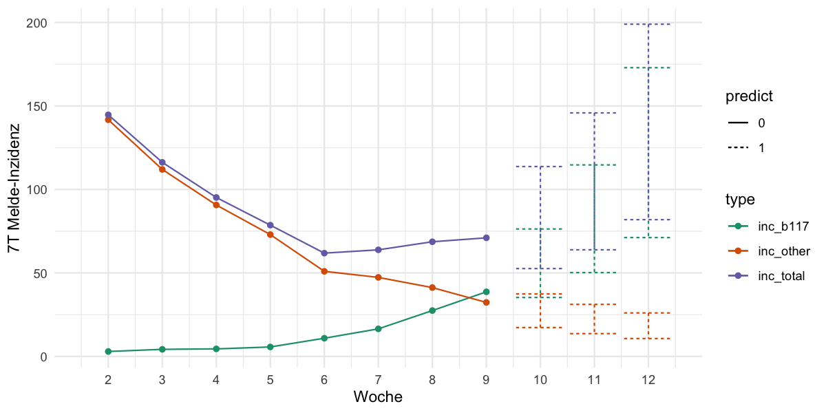
| #Plot the new version | |
| ggplot(df_plot, aes(x=kw, y=inc, color=type, linetype=predict)) + | |
| geom_line() + | |
| geom_point() + | |
| xlab("Woche") + ylab("7T Melde-Inzidenz") + | |
| geom_errorbar(aes(ymin=lower, ymax=upper)) + | |
| scale_color_brewer(palette = "Dark2") + | |
| scale_x_continuous(breaks=2:13) + | |
| theme_minimal() | |
| ggsave("exp.png", width=8, height=4, dpi=150) | |
| ################################################################## | |
| ## Compare results with AR(model) based on | |
| ## See https://otexts.com/fpp3/nonlinear-regression.html | |
| ## and https://otexts.com/fpp3/non-seasonal-arima.html | |
| ################################################################## | |
| library(fpp3) | |
| voc_ts <- voc_df_long %>% as_tsibble(index = "kw", key="type") | |
| # Fit models to each 'type' time series | |
| fit_trends <- voc_ts %>% | |
| model( | |
| `log(inc) ~ 1 + t + iid` = TSLM(log(inc) ~ 1 + trend()), | |
| `log(inc) ~ 1 + t + AR(1)` = ARIMA(log(inc) ~ 1 + trend() + pdq(1,0,0)) | |
| ) | |
| # Make a 4 week prediction | |
| fc_trends <- fit_trends %>% forecast(h = 3) | |
| fc <- fc_trends %>% hilo(level = c(95)) %>% unpack_hilo(cols="95%") | |
| # Show results | |
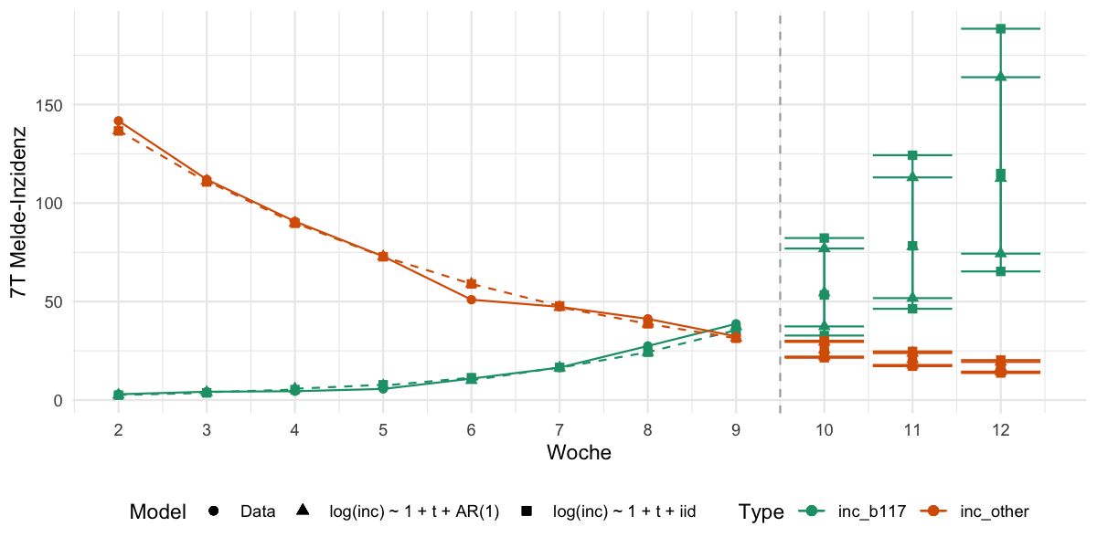
| afit <- augment(fit_trends) | |
| afit %>% | |
| ggplot(aes(x = kw)) + | |
| geom_line(data=voc_ts, aes(y = inc, colour = type)) + | |
| geom_point(data=voc_ts, aes(y = inc, colour = type, shape="Data"), size=2) + | |
| geom_line(aes(y = .fitted, colour = type), linetype=2) + | |
| geom_point(aes(y = .fitted, colour = type, shape=.model), size=2) + | |
| geom_errorbar(data=fc, aes(ymin=`95%_lower`,ymax= `95%_upper`,color=type)) + | |
| geom_point(data=fc, aes(y=.mean, color=type, shape=.model), size=2) + | |
| geom_point(data=fc, aes(y=`95%_lower`,color=type, shape=.model), size=2) + | |
| geom_point(data=fc, aes(y=`95%_upper`,color=type, shape=.model), size=2) + | |
| geom_vline(xintercept=9.5,lty=2, color="darkgray") + | |
| scale_color_brewer(palette = "Dark2") + | |
| guides(colour = guide_legend(title = "Type"), size = FALSE, shape=guide_legend(title="Model") ) + | |
| xlab("Woche") + ylab("7T Melde-Inzidenz") + | |
| scale_x_continuous(breaks=2:13) + | |
| theme_minimal() + | |
| theme(legend.position="bottom") | |
| ggsave("exp-expar.png", width=8, height=4, dpi=150) | |
Author
Sign up for free
to join this conversation on GitHub.
Already have an account?
Sign in to comment
2021-03-23 Original model (update: now as log(inc) ~ 1 + t)
2021-04-08 For comparison added a time series based approach, which allows the residuals of the log(inc) ~ 1 + t to be auto-correlated according to an AR(1) process.